Gradient Descent
Outline:
- Learning weights
- Gradient Descent
- Gradient Descent Math
- Gradient Descent Code
- Gradient Descent Implementation
- Reference
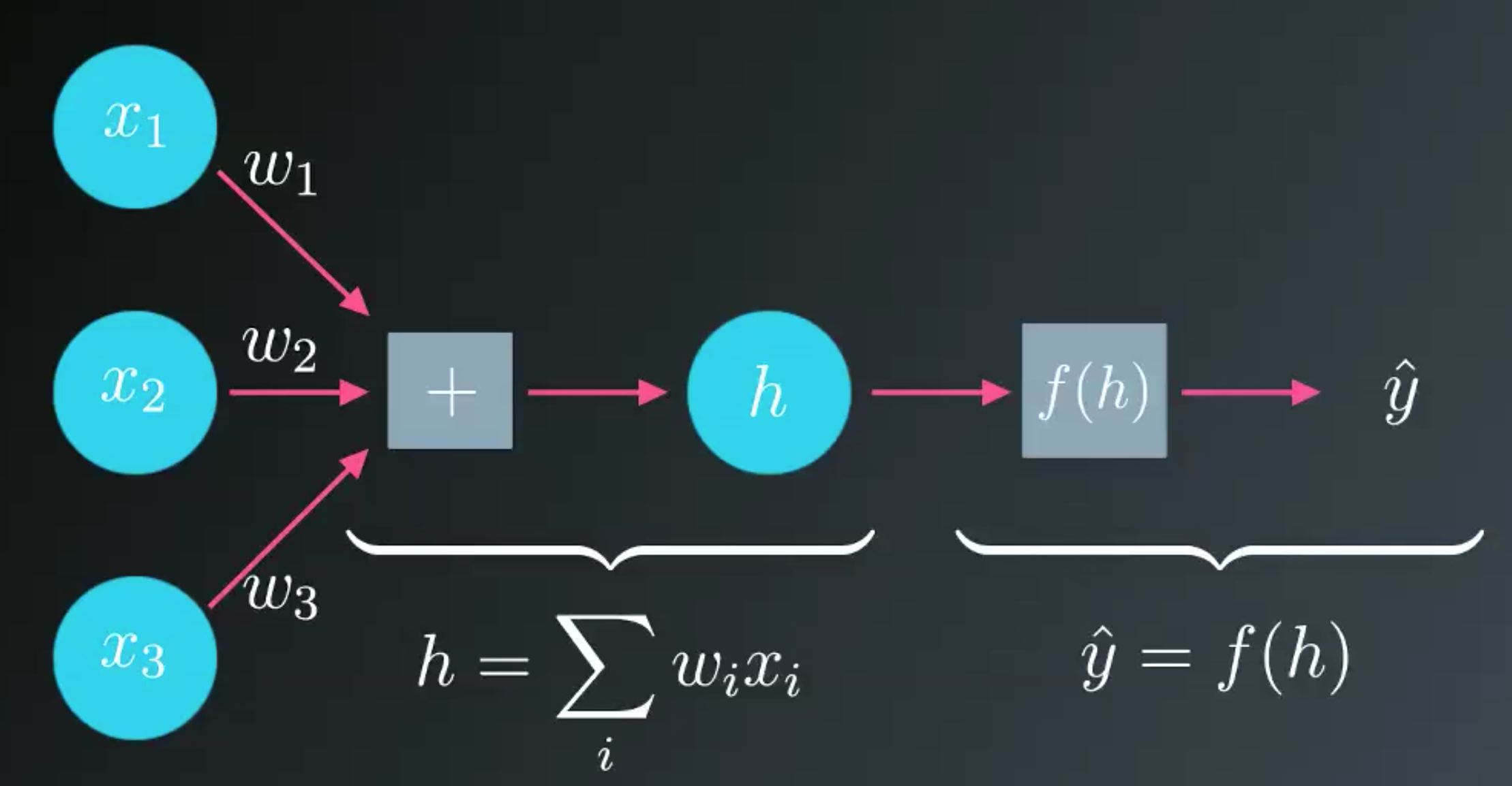
Learning weights
- We’ll need to learn the weights from example data, then use those weights to make the predictions.
- We want the network to make predictions as close as possible to the real values.
- To measure this, we need a metric of how wrong the predictions are, the error.
Error function
A common metric is the sum of the squared errors (SSE):
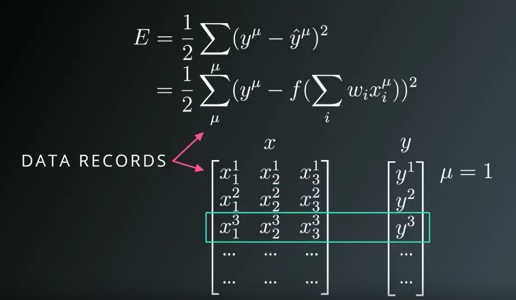
- We want the network’s prediction error to be as small as possible and the weights are the knobs we can use to make that happen.
- Our goal is to find weights that minimize the squared error .
- To do this with a neural network, typically you’d use gradient descent.
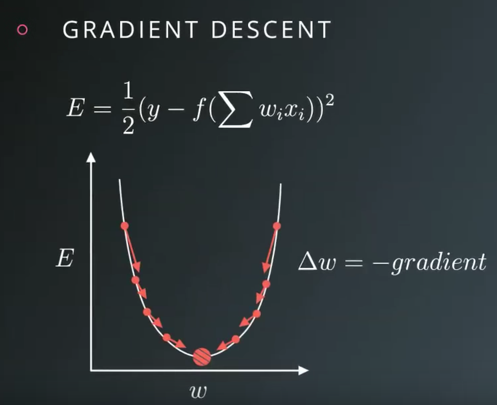
Gradient Descent
- With gradient descent, we take multiple small steps towards our goal.
- We want to change the weights in steps that reduce the error.
- The gradient is just a derivative generalized to functions with more than one variable.
- We can use calculus to find the gradient at any point in our error function, which depends on the input weights.
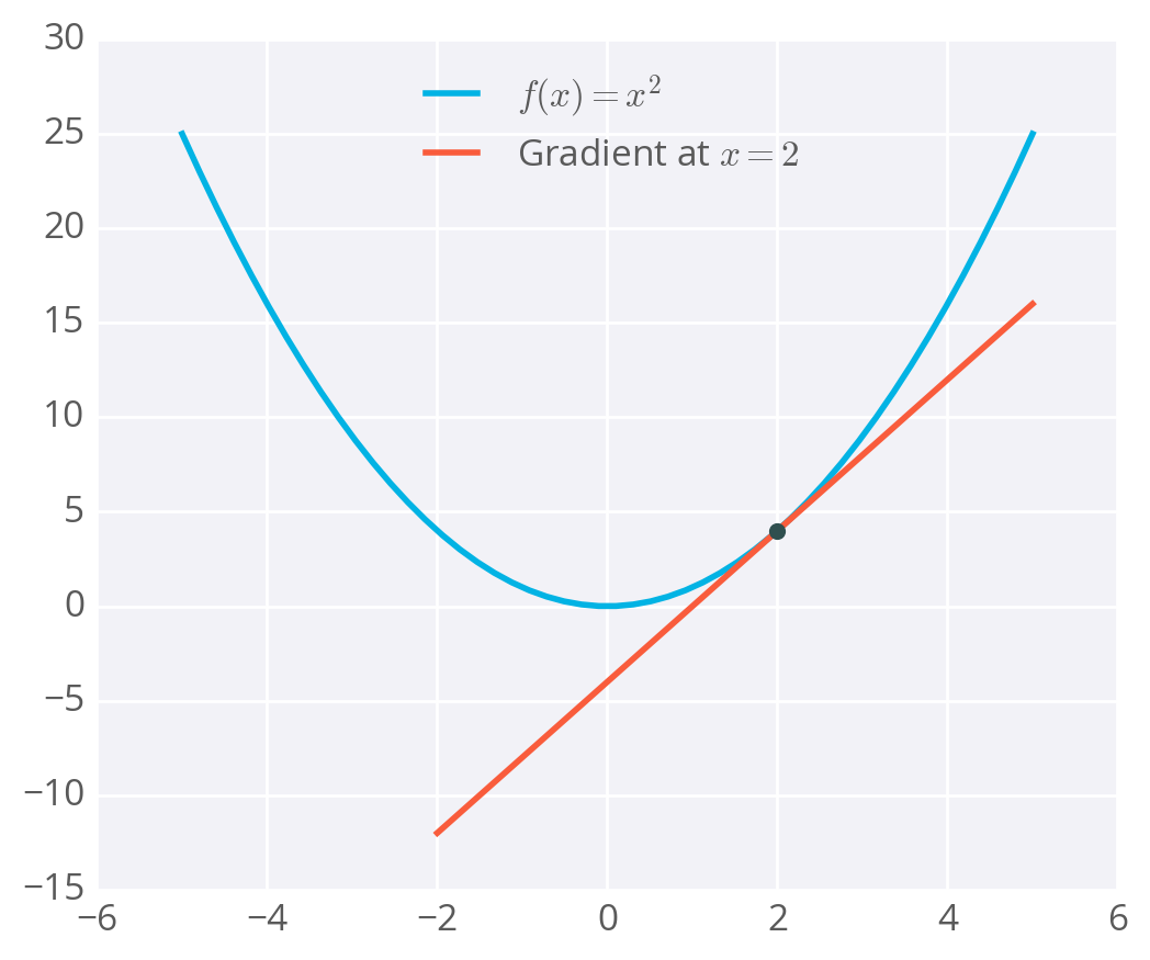
Derivative example
- The derivative of is .
- So, at , the slope is .
- Plotting this out, it looks like:
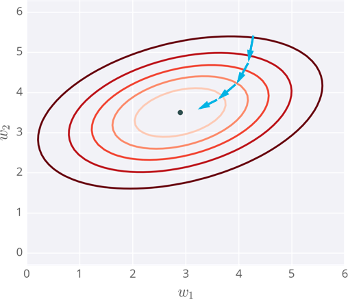
Contour Map
- Example of the error of a neural network with two inputs, and accordingly, two weights.
- At each step, you calculate the error and the gradient.
- Then use those to determine how much to change each weight.
- Repeating this process will eventually find weights that are close to the minimum of the error function, the block dot in the middle.
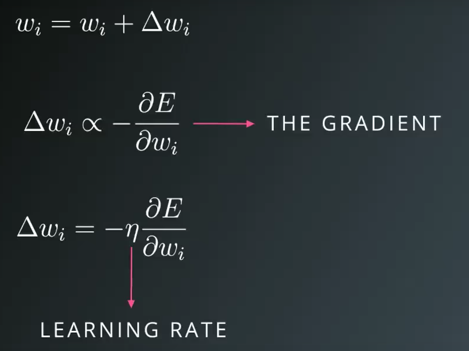
Gradient Descent Math
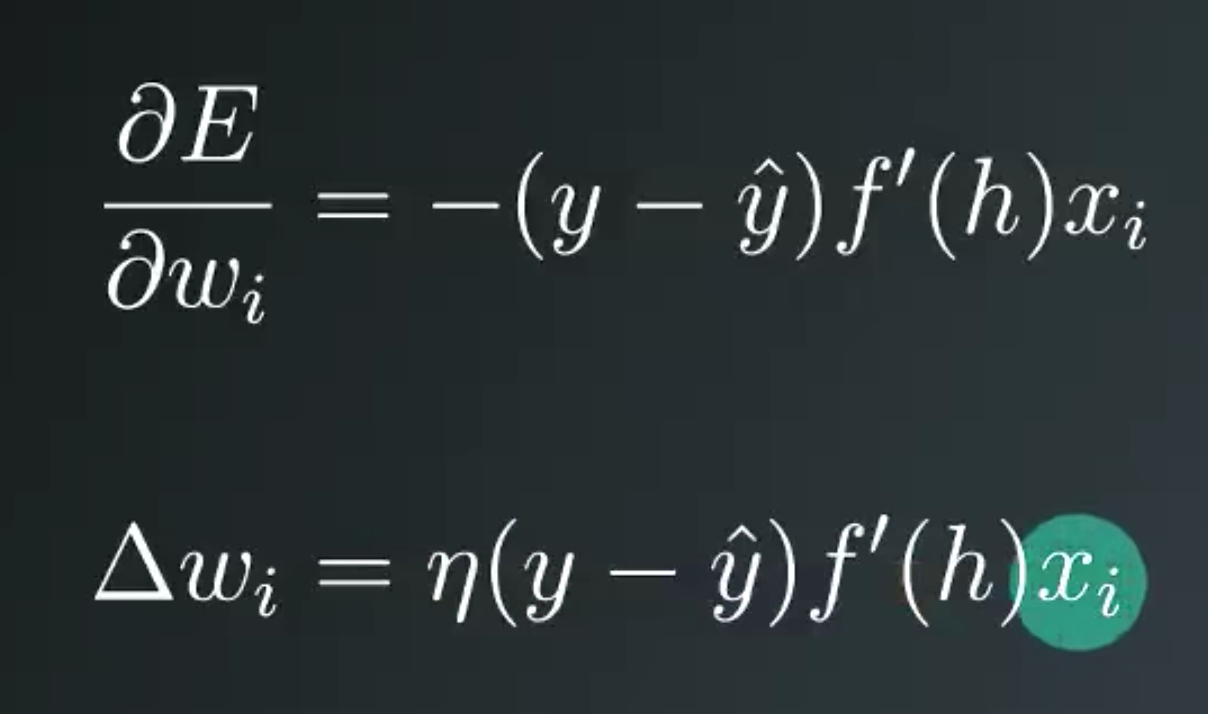
Learning Rate
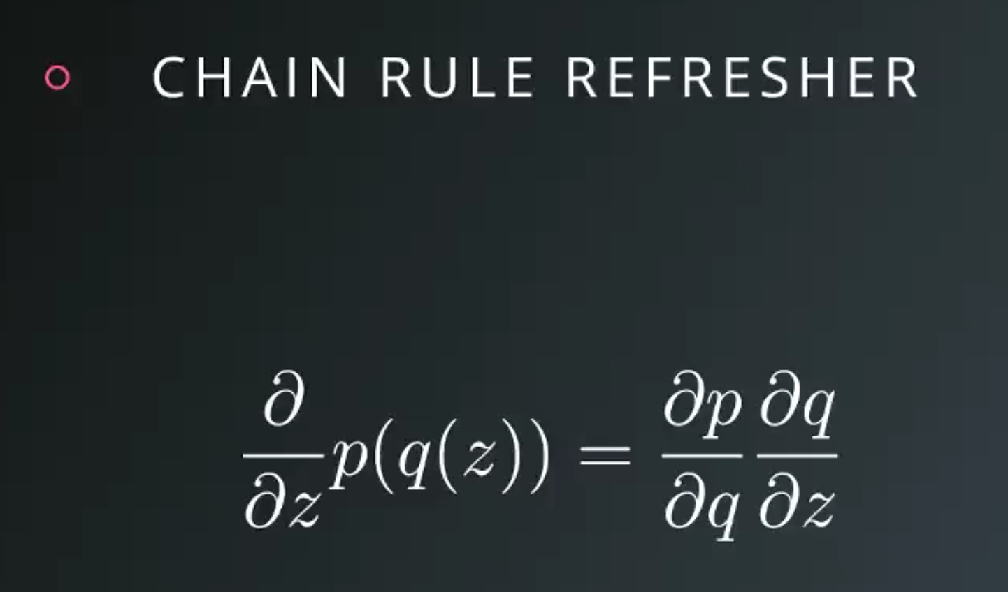
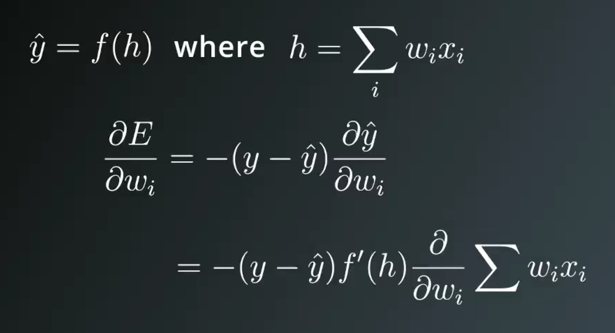
Chain Rule
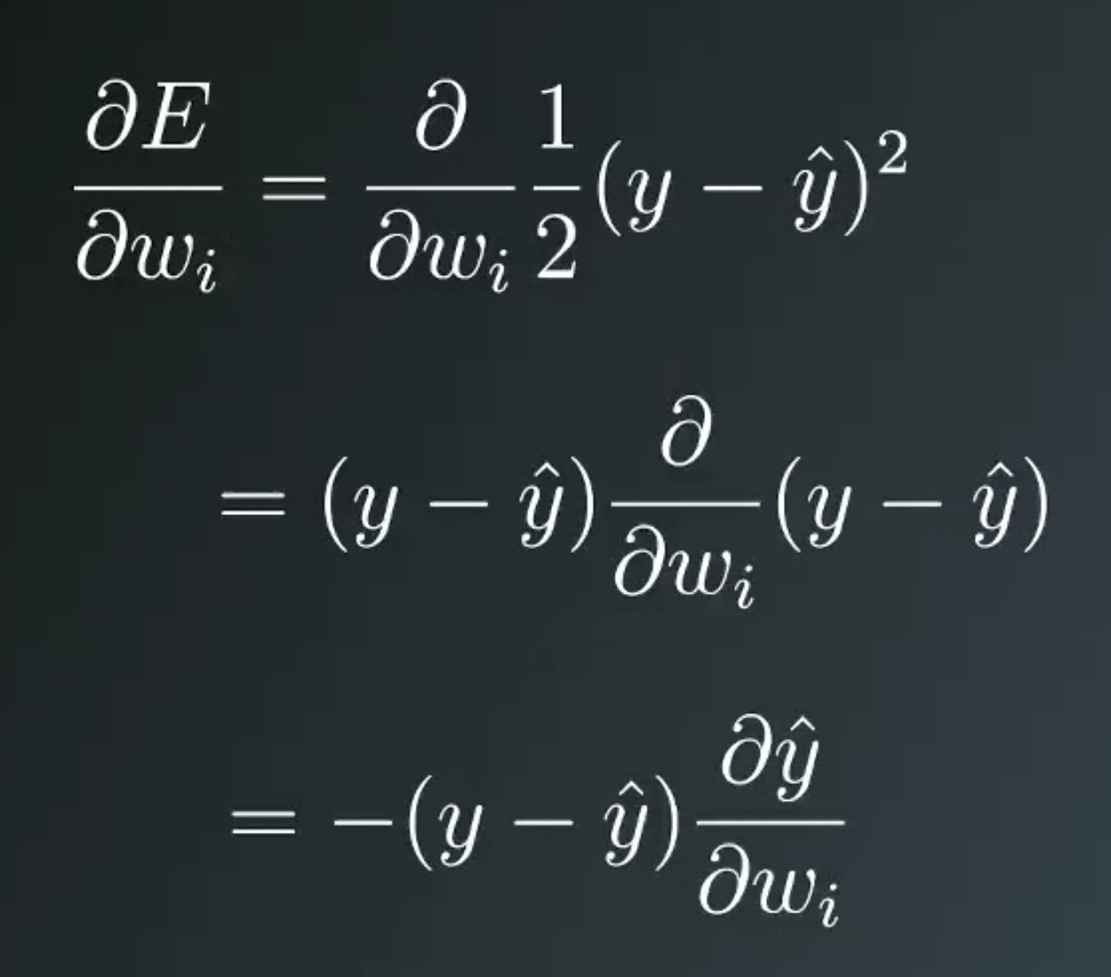
Derivative
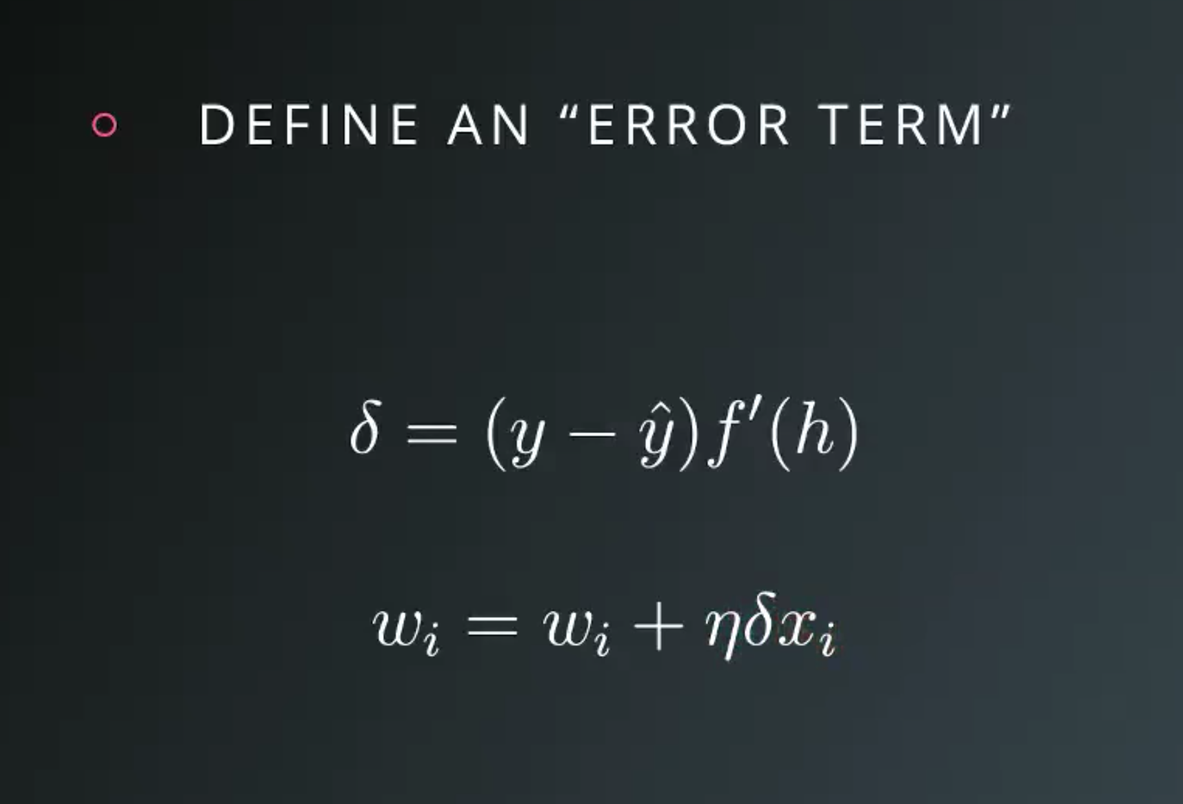
Define error term
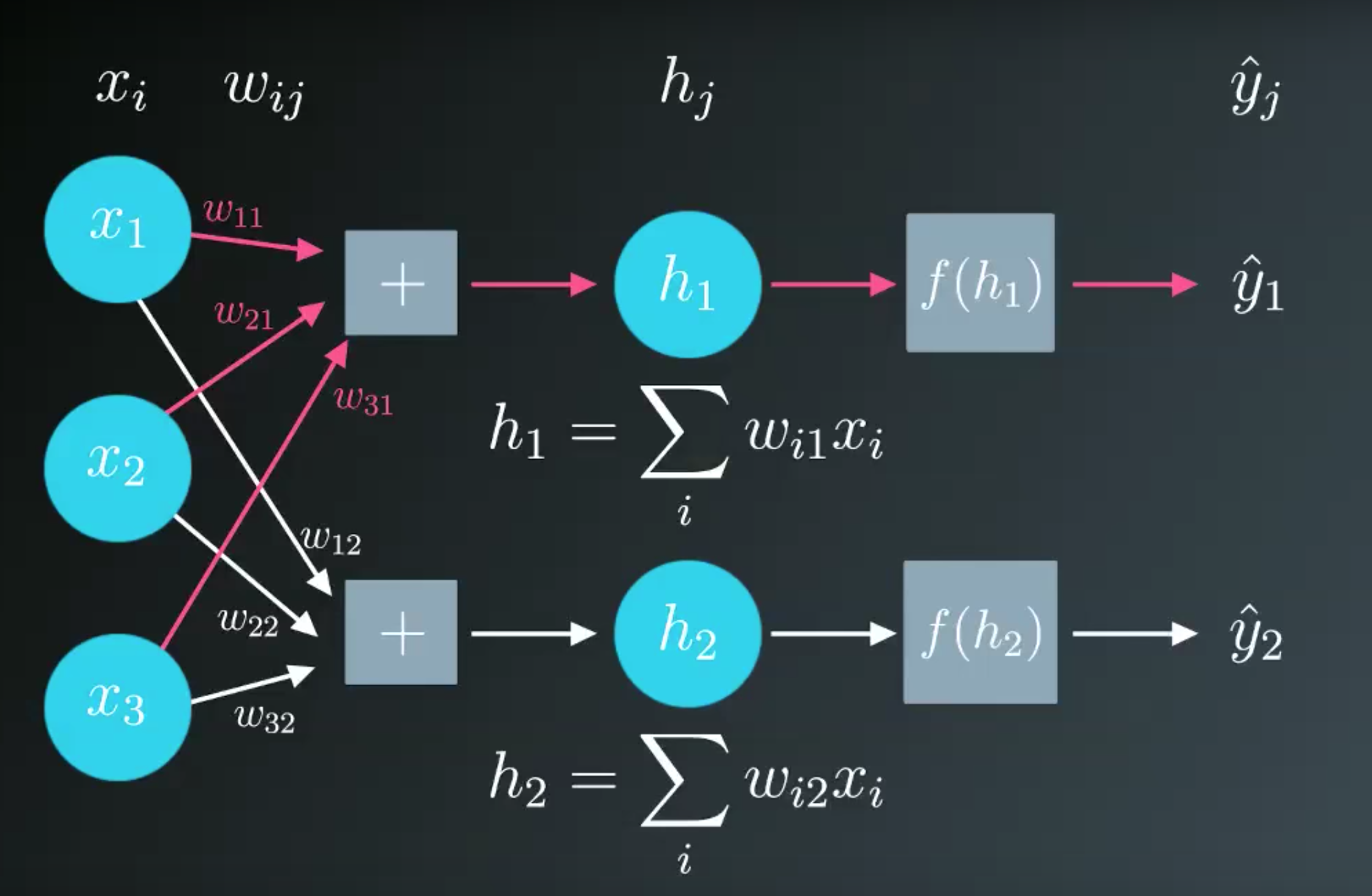
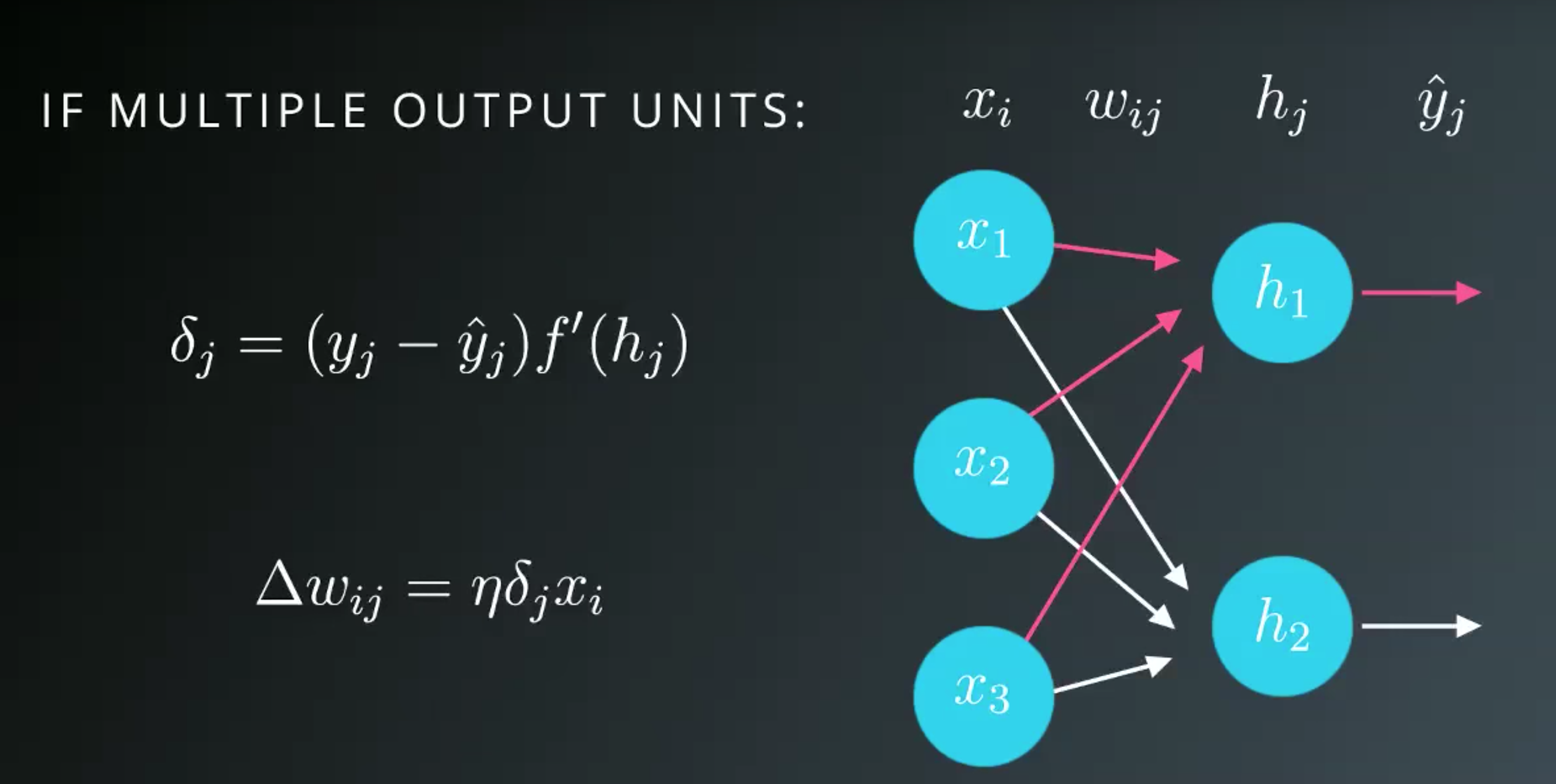
Multiple Outpus
Gradient Descent Code
- This code is for the case of only one output unit.
- We’ll also be using the sigmoid as the activation function
Code:
import numpy as np

def sigmoid(x):
    """
    Calculate sigmoid
    """
    return 1/(1+np.exp(-x))

def sigmoid_prime(x):
    """
    # Derivative of the sigmoid function
    """
    return sigmoid(x) * (1 - sigmoid(x))

learnrate = 0.5
x = np.array([1, 2, 3, 4])
y = np.array(0.5)

# Initial weights
w = np.array([0.5, -0.5, 0.3, 0.1])

### Calculate one gradient descent step for each weight
### Note: Some steps have been consilated, so there are
###       fewer variable names than in the above sample code

# TODO: Calculate the node's linear combination of inputs and weights
h = np.dot(x, w)

# TODO: Calculate output of neural network
nn_output = sigmoid(h)

# TODO: Calculate error of neural network
error = y - nn_output

# TODO: Calculate the error term
#       Remember, this requires the output gradient, which we haven't
#       specifically added a variable for.
error_term = error * sigmoid_prime(h)

# TODO: Calculate change in weights
del_w = learnrate * error_term * x

print('Neural Network output:')
print(nn_output)
print('Amount of Error:')
print(error)
print('Change in Weights:')
print(del_w)
Output:
Neural Network output:
0.689974481128
Amount of Error:
-0.189974481128
Change in Weights:
[-0.02031869 -0.04063738 -0.06095608 -0.08127477]
Gradient Descent Implementation
How do we translate that code to calculate many weight updates so our network will learn?
Example Scene
- Use gradient descent to train a network on graduate school admissions data
- This dataset has three input features:
- GRE score
- GPA
- Rank of the undergraduate school (numbered 1 through 4)
- Institutions with rank 1 have the highest prestige, those with rank 4 have the lowest.
- The goal here is to predict if a student will be admitted to a graduates program based on these features.
- Network with one output layer with one unit.
- Sigmoid function for the output unit activation.
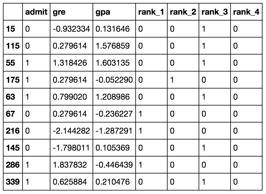
Data Cleanup
- The
rankfeature is categorical.- use dummy variables to encode
rank
- use dummy variables to encode
- To standardize the
GREandGPAdata- to scale the values such they have zero mean and a standard deviation of 1.
data_prep.py:
import numpy as np
import pandas as pd

admissions = pd.read_csv('binary.csv')

# Make dummy variables for rank
data = pd.concat([admissions, pd.get_dummies(admissions['rank'], prefix='rank')], axis=1)
data = data.drop('rank', axis=1)

# Standarize features
for field in ['gre', 'gpa']:
    mean, std = data[field].mean(), data[field].std()
    data.loc[:,field] = (data[field]-mean)/std

# Split off random 10% of the data for testing
np.random.seed(42)
sample = np.random.choice(data.index, size=int(len(data)*0.9), replace=False)
data, test_data = data.ix[sample], data.drop(sample)

# Split into features and targets
features, targets = data.drop('admit', axis=1), data['admit']
features_test, targets_test = test_data.drop('admit', axis=1), test_data['admit']
Implementation
Code:
import numpy as np
from data_prep import features, targets, features_test, targets_test


def sigmoid(x):
    """
    Calculate sigmoid
    """
    return 1 / (1 + np.exp(-x))

# TODO: We haven't provided the sigmoid_prime function like we did in
#       the previous lesson to encourage you to come up with a more
#       efficient solution. If you need a hint, check out the comments
#       in solution.py from the previous lecture.

# Use to same seed to make debugging easier
np.random.seed(42)

n_records, n_features = features.shape
last_loss = None

# Initialize weights
weights = np.random.normal(scale=1 / n_features**.5, size=n_features)

# Neural Network hyperparameters
epochs = 1000
learnrate = 0.5

for e in range(epochs):
    del_w = np.zeros(weights.shape)
    for x, y in zip(features.values, targets):
        # Loop through all records, x is the input, y is the target

        # Activation of the output unit
        #   Notice we multiply the inputs and the weights here
        #   rather than storing h as a separate variable
        output = sigmoid(np.dot(x, weights))

        # The error, the target minus the network output
        error = y - output

        # The error term
        #   Notice we calulate f'(h) here instead of defining a separate
        #   sigmoid_prime function. This just makes it faster because we
        #   can re-use the result of the sigmoid function stored in
        #   the output variable
        error_term = error * output * (1 - output)

        # The gradient descent step, the error times the gradient times the inputs
        del_w += error_term * x

    # Update the weights here. The learning rate times the
    # change in weights, divided by the number of records to average
    weights += learnrate * del_w / n_records

    # Printing out the mean square error on the training set
    if e % (epochs / 10) == 0:
        out = sigmoid(np.dot(features, weights))
        loss = np.mean((out - targets) ** 2)
        if last_loss and last_loss < loss:
            print("Train loss: ", loss, "  WARNING - Loss Increasing")
        else:
            print("Train loss: ", loss)
        last_loss = loss


# Calculate accuracy on test data
tes_out = sigmoid(np.dot(features_test, weights))
predictions = tes_out > 0.5
accuracy = np.mean(predictions == targets_test)
print("Prediction accuracy: {:.3f}".format(accuracy))
Output:
Train loss:  0.26276093849966364
Train loss:  0.20928619409324895
Train loss:  0.20084292908073417
Train loss:  0.19862156475527884
Train loss:  0.19779851396686018
Train loss:  0.19742577912189863
Train loss:  0.19723507746241065
Train loss:  0.19712945625092465
Train loss:  0.19706766341315074
Train loss:  0.19703005801777368
Prediction accuracy: 0.725