MiniFlow
Outline:
What is a Neural Network
- A neural network is a graph of mathematical functions:
- linear combinations and activation functions.
- The graph consists of nodes, and edges.
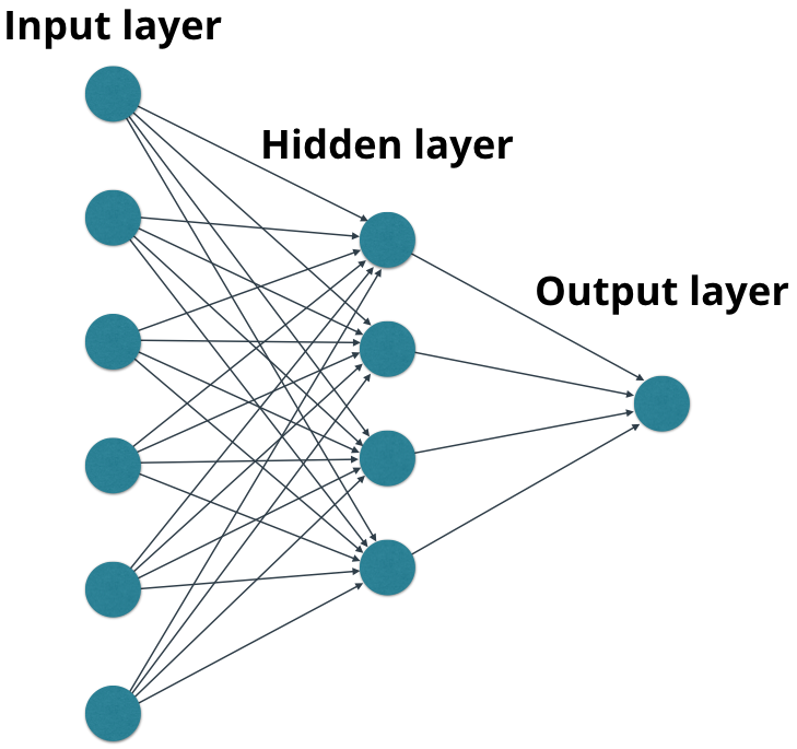
- Nodes in each layer (except for nodes in the input layer) perform mathematical functions using inputs from nodes in the previous layers.
- For example, a node could represent , where and are input values from nodes in the previous layer.
- Each node creates an output value which may be passed to nodes in the next layer.
- The output value from the output layer does not get passed to a future layer (last layer!)
- Layers between the input layer and the output layer are called hidden layers.
- The edges in the graph describe the connections between the nodes, along which the values flow from one layer to the next.
- These edges can also apply operations to the values that flow along them, such as multiplying by weights, adding biases, etc..
Graphs
- The nodes and edges create a graph structure.
- It isn’t hard to imagine that increasingly complex graphs can calculate almost anything.
- There are generally two steps to create neural networks:
- Define the graph of nodes and edges.
- Propagate values through the graph.
Gradient Descent
- Technically, the gradient actually points uphill, in the direction of steepest ascent.
- But if we put a
-sign in front of this value, we get the direction of steepest descent, which is what we want. - How much force should be applied to the push. This is known as the learning rate.
- which is an apt name since this value determines how quickly or slowly the neural network learns.
- This is more of a guessing game than anything else but empirically values in the range 0.1 to 0.0001 work well.
- The range 0.001 to 0.0001 is popular, as 0.1 and 0.01 are sometimes too large.
Gradient-Descent-Convergence:
Gradient-Descent-Civergence:

Code:
"""
Given the starting point of any `x` gradient descent
should be able to find the minimum value of x for the
cost function `f` defined below.
"""
import random
from gd import gradient_descent_update


def f(x):
    """
    Quadratic function.

    It's easy to see the minimum value of the function
    is 5 when is x=0.
    """
    return x**2 + 5


def df(x):
    """
    Derivative of `f` with respect to `x`.
    """
    return 2*x

def gradient_descent_update(x, gradx, learning_rate):
    """
    Performs a gradient descent update.
    """
    # TODO: Implement gradient descent.

    # Return the new value for x
    return x - learning_rate * gradx

# Random number between 0 and 10,000. Feel free to set x whatever you like.
x = random.randint(0, 10000)
# TODO: Set the learning rate
learning_rate = 0.1
epochs = 100

for i in range(epochs+1):
    cost = f(x)
    gradx = df(x)
    print("EPOCH {}: Cost = {:.3f}, x = {:.3f}".format(i, cost, gradx))
    x = gradient_descent_update(x, gradx, learning_rate)
Output:
EPOCH 0: Cost = 2601774.000, x = 3226.000
EPOCH 1: Cost = 1665137.160, x = 2580.800
EPOCH 2: Cost = 1065689.582, x = 2064.640
EPOCH 3: Cost = 682043.133, x = 1651.712
EPOCH 4: Cost = 436509.405, x = 1321.370
EPOCH 5: Cost = 279367.819, x = 1057.096
EPOCH 6: Cost = 178797.204, x = 845.677
EPOCH 7: Cost = 114432.011, x = 676.541
EPOCH 8: Cost = 73238.287, x = 541.233
EPOCH 9: Cost = 46874.304, x = 432.986
EPOCH 10: Cost = 30001.354, x = 346.389
EPOCH 11: Cost = 19202.667, x = 277.111
EPOCH 12: Cost = 12291.507, x = 221.689
EPOCH 13: Cost = 7868.364, x = 177.351
EPOCH 14: Cost = 5037.553, x = 141.881
EPOCH 15: Cost = 3225.834, x = 113.505
EPOCH 16: Cost = 2066.334, x = 90.804
EPOCH 17: Cost = 1324.254, x = 72.643
EPOCH 18: Cost = 849.322, x = 58.114
EPOCH 19: Cost = 545.366, x = 46.492
EPOCH 20: Cost = 350.834, x = 37.193
EPOCH 21: Cost = 226.334, x = 29.755
EPOCH 22: Cost = 146.654, x = 23.804
EPOCH 23: Cost = 95.658, x = 19.043
EPOCH 24: Cost = 63.021, x = 15.234
EPOCH 25: Cost = 42.134, x = 12.187
EPOCH 26: Cost = 28.766, x = 9.750
EPOCH 27: Cost = 20.210, x = 7.800
EPOCH 28: Cost = 14.734, x = 6.240
EPOCH 29: Cost = 11.230, x = 4.992
EPOCH 30: Cost = 8.987, x = 3.994
EPOCH 31: Cost = 7.552, x = 3.195
EPOCH 32: Cost = 6.633, x = 2.556
EPOCH 33: Cost = 6.045, x = 2.045
EPOCH 34: Cost = 5.669, x = 1.636
EPOCH 35: Cost = 5.428, x = 1.309
EPOCH 36: Cost = 5.274, x = 1.047
EPOCH 37: Cost = 5.175, x = 0.838
EPOCH 38: Cost = 5.112, x = 0.670
EPOCH 39: Cost = 5.072, x = 0.536
EPOCH 40: Cost = 5.046, x = 0.429
Stochastic Gradient Descent
- Stochastic Gradient Descent (SGD) is a version of Gradient Descent
- Where on each forward pass a batch of data is randomly sampled from total dataset.
- Ideally, the entire dataset would be fed into the neural network on each forward pass.
- But in practice, it’s not practical due to memory constraints.
- SGD is an approximation of Gradient Descent.
- The more batches processed by the neural network, the better the approximation.
A naïve implementation of SGD involves:
- Randomly sample a batch of data from the total dataset.
- Running the network forward and backward to calculate the gradient (with data from (1)).
- Apply the gradient descent update.
- Repeat steps 1-3 until convergence or the loop is stopped by another mechanism (i.e. the number of epochs).
Code: miniflow.py
import numpy as np

class Node:
    """
    Base class for nodes in the network.

    Arguments:

        `inbound_nodes`: A list of nodes with edges into this node.
    """
    def __init__(self, inbound_nodes=[]):
        """
        Node's constructor (runs when the object is instantiated). Sets
        properties that all nodes need.
        """
        # A list of nodes with edges into this node.
        self.inbound_nodes = inbound_nodes
        # The eventual value of this node. Set by running
        # the forward() method.
        self.value = None
        # A list of nodes that this node outputs to.
        self.outbound_nodes = []
        # New property! Keys are the inputs to this node and
        # their values are the partials of this node with
        # respect to that input.
        self.gradients = {}
        # Sets this node as an outbound node for all of
        # this node's inputs.
        for node in inbound_nodes:
            node.outbound_nodes.append(self)

    def forward(self):
        """
        Every node that uses this class as a base class will
        need to define its own `forward` method.
        """
        raise NotImplementedError

    def backward(self):
        """
        Every node that uses this class as a base class will
        need to define its own `backward` method.
        """
        raise NotImplementedError


class Input(Node):
    """
    A generic input into the network.
    """
    def __init__(self):
        # The base class constructor has to run to set all
        # the properties here.
        #
        # The most important property on an Input is value.
        # self.value is set during `topological_sort` later.
        Node.__init__(self)

    def forward(self):
        # Do nothing because nothing is calculated.
        pass

    def backward(self):
        # An Input node has no inputs so the gradient (derivative)
        # is zero.
        # The key, `self`, is reference to this object.
        self.gradients = {self: 0}
        # Weights and bias may be inputs, so you need to sum
        # the gradient from output gradients.
        for n in self.outbound_nodes:
            self.gradients[self] += n.gradients[self]

class Linear(Node):
    """
    Represents a node that performs a linear transform.
    """
    def __init__(self, X, W, b):
        # The base class (Node) constructor. Weights and bias
        # are treated like inbound nodes.
        Node.__init__(self, [X, W, b])

    def forward(self):
        """
        Performs the math behind a linear transform.
        """
        X = self.inbound_nodes[0].value
        W = self.inbound_nodes[1].value
        b = self.inbound_nodes[2].value
        self.value = np.dot(X, W) + b

    def backward(self):
        """
        Calculates the gradient based on the output values.
        """
        # Initialize a partial for each of the inbound_nodes.
        self.gradients = {n: np.zeros_like(n.value) for n in self.inbound_nodes}
        # Cycle through the outputs. The gradient will change depending
        # on each output, so the gradients are summed over all outputs.
        for n in self.outbound_nodes:
            # Get the partial of the cost with respect to this node.
            grad_cost = n.gradients[self]
            # Set the partial of the loss with respect to this node's inputs.
            self.gradients[self.inbound_nodes[0]] += np.dot(grad_cost, self.inbound_nodes[1].value.T)
            # Set the partial of the loss with respect to this node's weights.
            self.gradients[self.inbound_nodes[1]] += np.dot(self.inbound_nodes[0].value.T, grad_cost)
            # Set the partial of the loss with respect to this node's bias.
            self.gradients[self.inbound_nodes[2]] += np.sum(grad_cost, axis=0, keepdims=False)


class Sigmoid(Node):
    """
    Represents a node that performs the sigmoid activation function.
    """
    def __init__(self, node):
        # The base class constructor.
        Node.__init__(self, [node])

    def _sigmoid(self, x):
        """
        This method is separate from `forward` because it
        will be used with `backward` as well.

        `x`: A numpy array-like object.
        """
        return 1. / (1. + np.exp(-x))

    def forward(self):
        """
        Perform the sigmoid function and set the value.
        """
        input_value = self.inbound_nodes[0].value
        self.value = self._sigmoid(input_value)

    def backward(self):
        """
        Calculates the gradient using the derivative of
        the sigmoid function.
        """
        # Initialize the gradients to 0.
        self.gradients = {n: np.zeros_like(n.value) for n in self.inbound_nodes}
        # Sum the partial with respect to the input over all the outputs.
        for n in self.outbound_nodes:
            grad_cost = n.gradients[self]
            sigmoid = self.value
            self.gradients[self.inbound_nodes[0]] += sigmoid * (1 - sigmoid) * grad_cost


class MSE(Node):
    def __init__(self, y, a):
        """
        The mean squared error cost function.
        Should be used as the last node for a network.
        """
        # Call the base class' constructor.
        Node.__init__(self, [y, a])

    def forward(self):
        """
        Calculates the mean squared error.
        """
        # NOTE: We reshape these to avoid possible matrix/vector broadcast
        # errors.
        #
        # For example, if we subtract an array of shape (3,) from an array of shape
        # (3,1) we get an array of shape(3,3) as the result when we want
        # an array of shape (3,1) instead.
        #
        # Making both arrays (3,1) insures the result is (3,1) and does
        # an elementwise subtraction as expected.
        y = self.inbound_nodes[0].value.reshape(-1, 1)
        a = self.inbound_nodes[1].value.reshape(-1, 1)

        self.m = self.inbound_nodes[0].value.shape[0]
        # Save the computed output for backward.
        self.diff = y - a
        self.value = np.mean(self.diff**2)

    def backward(self):
        """
        Calculates the gradient of the cost.
        """
        self.gradients[self.inbound_nodes[0]] = (2 / self.m) * self.diff
        self.gradients[self.inbound_nodes[1]] = (-2 / self.m) * self.diff


def topological_sort(feed_dict):
    """
    Sort the nodes in topological order using Kahn's Algorithm.

    `feed_dict`: A dictionary where the key is a `Input` Node and the value is the respective value feed to that Node.

    Returns a list of sorted nodes.
    """

    input_nodes = [n for n in feed_dict.keys()]

    G = {}
    nodes = [n for n in input_nodes]
    while len(nodes) > 0:
        n = nodes.pop(0)
        if n not in G:
            G[n] = {'in': set(), 'out': set()}
        for m in n.outbound_nodes:
            if m not in G:
                G[m] = {'in': set(), 'out': set()}
            G[n]['out'].add(m)
            G[m]['in'].add(n)
            nodes.append(m)

    L = []
    S = set(input_nodes)
    while len(S) > 0:
        n = S.pop()

        if isinstance(n, Input):
            n.value = feed_dict[n]

        L.append(n)
        for m in n.outbound_nodes:
            G[n]['out'].remove(m)
            G[m]['in'].remove(n)
            # if no other incoming edges add to S
            if len(G[m]['in']) == 0:
                S.add(m)
    return L


def forward_and_backward(graph):
    """
    Performs a forward pass and a backward pass through a list of sorted Nodes.

    Arguments:

        `graph`: The result of calling `topological_sort`.
    """
    # Forward pass
    for n in graph:
        n.forward()

    # Backward pass
    # see: https://docs.python.org/2.3/whatsnew/section-slices.html
    for n in graph[::-1]:
        n.backward()


def sgd_update(trainables, learning_rate=1e-2):
    """
    Updates the value of each trainable with SGD.

    Arguments:

        `trainables`: A list of `Input` Nodes representing weights/biases.
        `learning_rate`: The learning rate.
    """
    # Performs SGD
    #
    # Loop over the trainables
    for t in trainables:
        # Change the trainable's value by subtracting the learning rate
        # multiplied by the partial of the cost with respect to this
        # trainable.
        partial = t.gradients[t]
        t.value -= learning_rate * partial
Code: nn.py
"""
Have fun with the number of epochs!

Be warned that if you increase them too much,
the VM will time out :)
"""

import numpy as np
from sklearn.datasets import load_boston
from sklearn.utils import shuffle, resample
from miniflow import *

# Load data
data = load_boston()
X_ = data['data']
y_ = data['target']

# Normalize data
X_ = (X_ - np.mean(X_, axis=0)) / np.std(X_, axis=0)

n_features = X_.shape[1]
n_hidden = 10
W1_ = np.random.randn(n_features, n_hidden)
b1_ = np.zeros(n_hidden)
W2_ = np.random.randn(n_hidden, 1)
b2_ = np.zeros(1)

# Neural network
X, y = Input(), Input()
W1, b1 = Input(), Input()
W2, b2 = Input(), Input()

l1 = Linear(X, W1, b1)
s1 = Sigmoid(l1)
l2 = Linear(s1, W2, b2)
cost = MSE(y, l2)

feed_dict = {
    X: X_,
    y: y_,
    W1: W1_,
    b1: b1_,
    W2: W2_,
    b2: b2_
}

epochs = 10
# Total number of examples
m = X_.shape[0]
batch_size = 11
steps_per_epoch = m // batch_size

graph = topological_sort(feed_dict)
trainables = [W1, b1, W2, b2]

print("Total number of examples = {}".format(m))

# Step 4
for i in range(epochs):
    loss = 0
    for j in range(steps_per_epoch):
        # Step 1
        # Randomly sample a batch of examples
        X_batch, y_batch = resample(X_, y_, n_samples=batch_size)

        # Reset value of X and y Inputs
        X.value = X_batch
        y.value = y_batch

        # Step 2
        forward_and_backward(graph)

        # Step 3
        sgd_update(trainables)

        loss += graph[-1].value

    print("Epoch: {}, Loss: {:.3f}".format(i+1, loss/steps_per_epoch))
Output:
Total number of examples = 506
Epoch: 1, Loss: 137.353
Epoch: 2, Loss: 38.041
Epoch: 3, Loss: 30.666
Epoch: 4, Loss: 24.717
Epoch: 5, Loss: 23.817
...
...
...
Epoch: 994, Loss: 3.993
Epoch: 995, Loss: 3.549
Epoch: 996, Loss: 4.550
Epoch: 997, Loss: 3.830
Epoch: 998, Loss: 3.975
Epoch: 999, Loss: 3.160
Epoch: 1000, Loss: 3.711