Intro to Tensorflow
Outline:
- Installing TensorFlow
- Hello, Tensor World!
- TensorFlow Input
- TensorFlow Math
- TensorFlow Linear Function
- ReLU and Softmax Activation Functions
- Softmax
- One-Hot Encoding
- Categorical Cross-Entropy
- Minimizing Cross Entropy
- Normalized Inputs and Initial Weights
- Measuring Performance
- Stochastic Gradient Descent
- Mini-Batch
Installing TensorFlow
OS X or Linux
conda create -n tensorflow python=3.5
source activate tensorflow
conda install pandas matplotlib jupyter notebook scipy scikit-learn
pip install tensorflow
Hello World!
import tensorflow as tf

# Create TensorFlow object called tensor
hello_constant = tf.constant('Hello World!')

with tf.Session() as sess:
    # Run the tf.constant operation in the session
    output = sess.run(hello_constant)
    print(output)
Hello, Tensor World!
Tensor
- In TensorFlow, data isn’t stored as integers, floats, or strings.
- These values are encapsulated in an object called a tensor.
- In the case of
hello_constant = tf.constant('Hello World!')hello_constantis a 0-dimensional string tensor
- Tensors come in a variety of sizes as shown below:
# A is a 0-dimensional int32 tensor A = tf.constant(1234) # B is a 1-dimensional int32 tensor B = tf.constant([123,456,789]) # C is a 2-dimensional int32 tensor C = tf.constant([ [123,456,789], [222,333,444] ]) - The tensor returned by
tf.constant()is called a constant tensor.- Because the value of the tensor never changes.
Session
- TensorFlow’s api is built around the idea of a computational graph, a way of visualizing a mathematical process.
- TensorFlow code you ran and turn that into a graph:
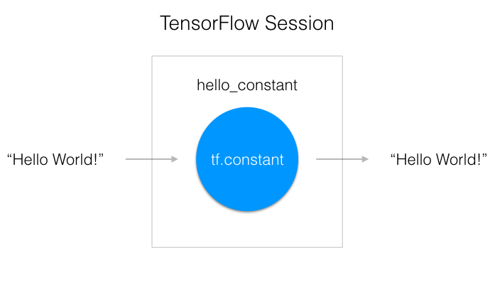
- A TensorFlow Session, as shown above, is an environment for running a graph.
- The session is in charge of allocating the operations to GPU(s) and/or CPU(s), including remote machines.
Example:
with tf.Session() as sess:
    output = sess.run(hello_constant)
    print(output)
- The code has already created the tensor,
hello_constant, from the previous lines. - The next step is to evaluate the tensor in a session.
- The code creates a session instance, sess, using
tf.Session. - The
sess.run()function then evaluates the tensor and returns the results.
Output:
'Hello World!'
TensorFlow Input
Placeholder
- We can’t just set
xto our dataset and put it in TensorFlow.- Because over time we’ll want our TensorFlow model to take in different datasets with different parameters.
tf.placeholder()returns a tensor that gets its value from data passed to thetf.session.run()function.- Allowing we to set the input right before the session runs.
Session’s feed
x = tf.placeholder(tf.string)

with tf.Session() as sess:
    output = sess.run(x, feed_dict={x: 'Hello World'})
- Use the
feed_dictparameter intf.session.run()to set the placeholder tensor. - The above example shows the tensor
xbeing set to the string"Hello, world". - It’s also possible to set more than one tensor using
feed_dictas shown below.x = tf.placeholder(tf.string) y = tf.placeholder(tf.int32) z = tf.placeholder(tf.float32) with tf.Session() as sess: output = sess.run(x, feed_dict={x: 'Test String', y: 123, z: 45.67})
TensorFlow Math
import tensorflow as tf

# TODO: Convert the following to TensorFlow:
x = tf.constant(10)  # x = 10
y = tf.constant(2)  # y = 2
z = tf.subtract(tf.divide(x,y),tf.cast(tf.constant(1), tf.float64))  # z = x/y - 1

# TODO: Print z from a session
with tf.Session() as sess:
    output = sess.run(z)
    print(output)
TensorFlow Linear Function
- W is a matrix of the weights connecting two layers.
- The output y, the input x, and the biases b are all vectors.
Weights and Bias in TensorFlow
- The
tf.Variableclass creates a tensor with an initial value that can be modified, much like a normal Python variable. - This tensor stores its state in the session, so you must initialize the state of the tensor manually.
- You’ll use the
tf.global_variables_initializer()function to initialize the state of all the Variable tensors.x = tf.Variable(5) init = tf.global_variables_initializer() with tf.Session() as sess: sess.run(init) tf.truncated_normal()function returns a tensor with random values from a normal distribution whose magnitude is no more than 2 standard deviations from the mean.n_features = 120 n_labels = 5 weights = tf.Variable(tf.truncated_normal((n_features, n_labels)))
ReLU and Softmax Activation Functions
- The sigmoid function as the activation function on our hidden units and, in the case of classification, on the output unit.
- However, this is not the only activation function you can use and actually has some drawbacks.
Sigmoid Functions
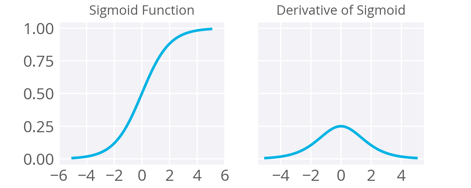
- As noted in the backpropagation, the derivative of the sigmoid maxes out at
0.25(see above). - This means when you’re performing backpropagation with sigmoid units, the errors going back into the network will be shrunk by at least
75%at every layer. - For layers close to the input layer, the weight updates will be tiny if you have a lot of layers and those weights will take a really long time to train.
- Due to this, sigmoids have fallen out of favor as activations on hidden units.
Enter Rectified Linear Units (ReLu)
- Most recent deep learning networks use rectified linear units (ReLUs) for the hidden layers.
- A rectified linear unit has output
0if the input is less than0, and raw output otherwise. - That is, if the input is greater than
0, the output is equal to the input. - Mathematically, that looks like:
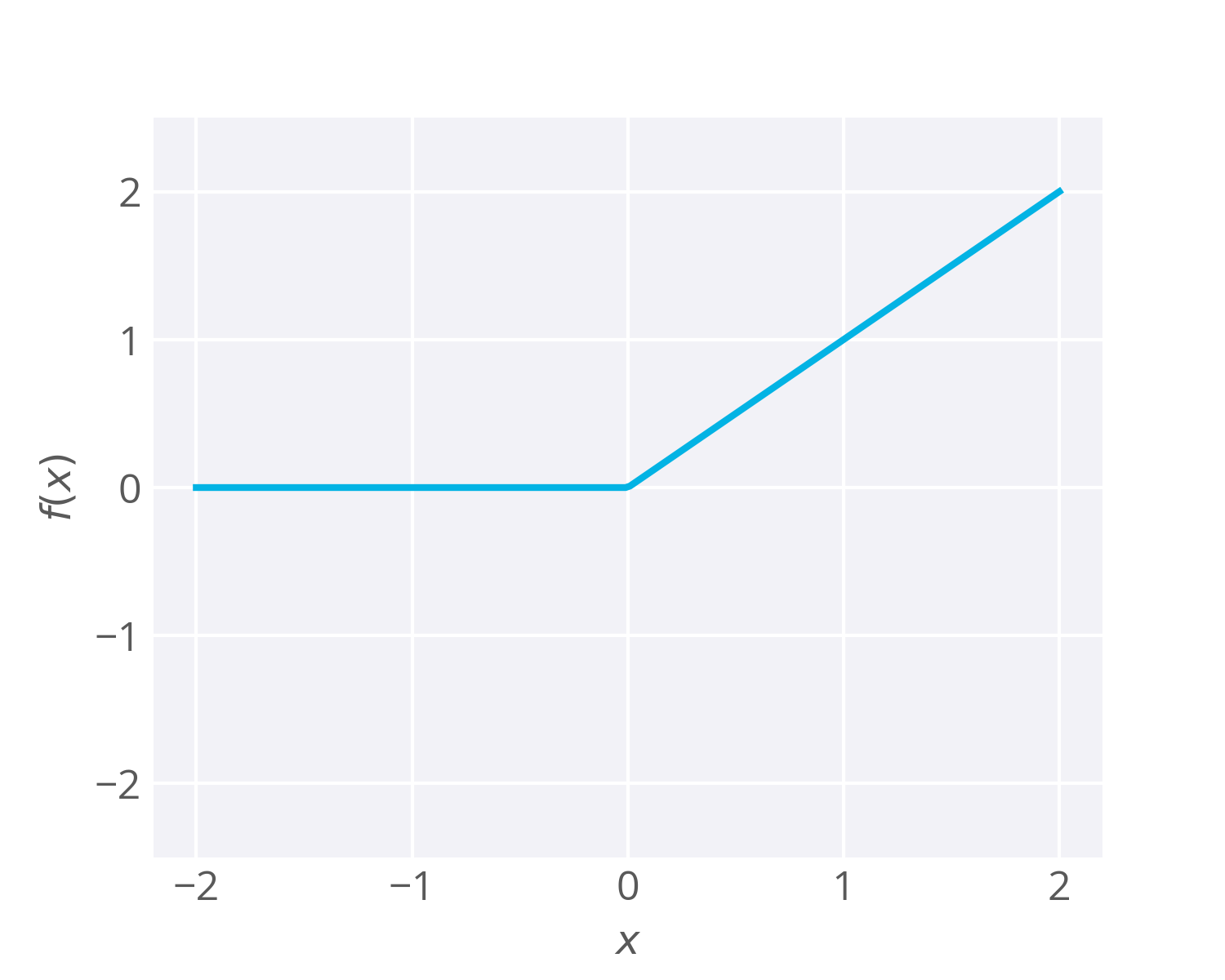
- ReLU activations are the simplest non-linear activation function you can use.
- When the input is positive, the derivative is
1.- So there isn’t the vanishing effect you see on backpropagated errors from sigmoids.
- Research has shown that ReLUs result in much faster training for large networks.
- Most frameworks like TensorFlow and TFLearn make it simple to use ReLUs on the the hidden layers, so you won’t need to implement them yourself.
Drawbacks
- It’s possible that a large gradient can set the weights such that a ReLU unit will always be
0. - These “dead” units will always be
0and a lot of computation will be wasted in training. - With a proper setting of the learning rate this is less frequently an issue.
Softmax
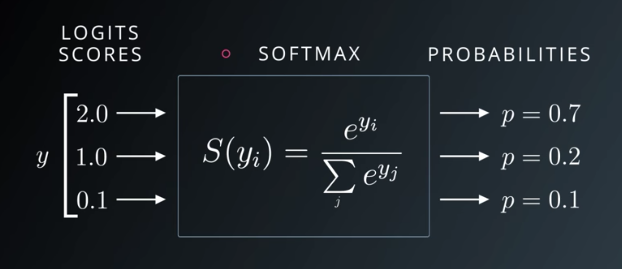
- The softmax function squashes the outputs of each unit to be between
0and1, just like a sigmoid. - It also divides each output such that the total sum of the outputs is equal to
1. - The output of the softmax function is equivalent to a categorical probability distribution.
- It tells you the probability that any of the classes are true.
The softmax can be used for any number of classes.
- Used to predict two classes of sentiment: positive or negative.
- Also used for hundreds and thousands of classes: object recognition problems where there are hundreds of different possible objects.
Tensorflow Softmax
import tensorflow as tf

output = None
logit_data = [2.0, 1.0, 0.1]
logits = tf.placeholder(tf.float32)

softmax = tf.nn.softmax(logits)

with tf.Session() as sess:
    output = sess.run(softmax, feed_dict={logits: logit_data})
logit is linear nodes.
One-Hot Encoding
- Transforming your labels into one-hot encoded vectors is pretty simple with scikit-learn using
LabelBinarizer.
import numpy as np
from sklearn import preprocessing

# Example labels
labels = np.array([1,5,3,2,1,4,2,1,3])

# Create the encoder
lb = preprocessing.LabelBinarizer()

# Here the encoder finds the classes and assigns one-hot vectors
lb.fit(labels)

# And finally, transform the labels into one-hot encoded vectors
lb.transform(labels)
>>> array([[1, 0, 0, 0, 0],
           [0, 0, 0, 0, 1],
           [0, 0, 1, 0, 0],
           [0, 1, 0, 0, 0],
           [1, 0, 0, 0, 0],
           [0, 0, 0, 1, 0],
           [0, 1, 0, 0, 0],
           [1, 0, 0, 0, 0],
           [0, 0, 1, 0, 0]])
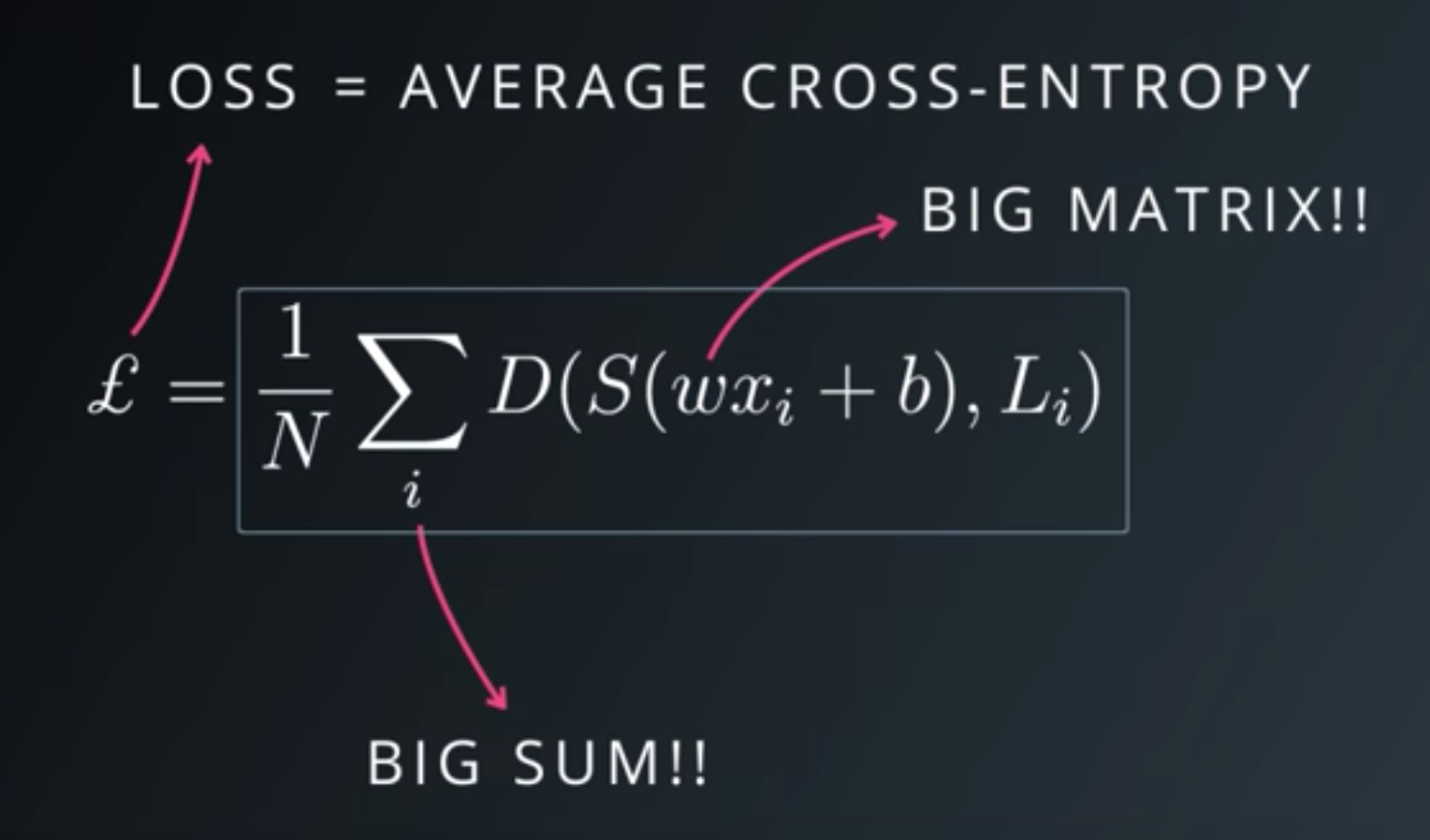
Categorical Cross-Entropy
- We’ve been using the sum of squared errors as the cost function in our networks.
- But in those cases we only have singular (scalar) output values.
- When you’re using softmax, however, your output is a vector.
- One vector is the probability values from the output units.
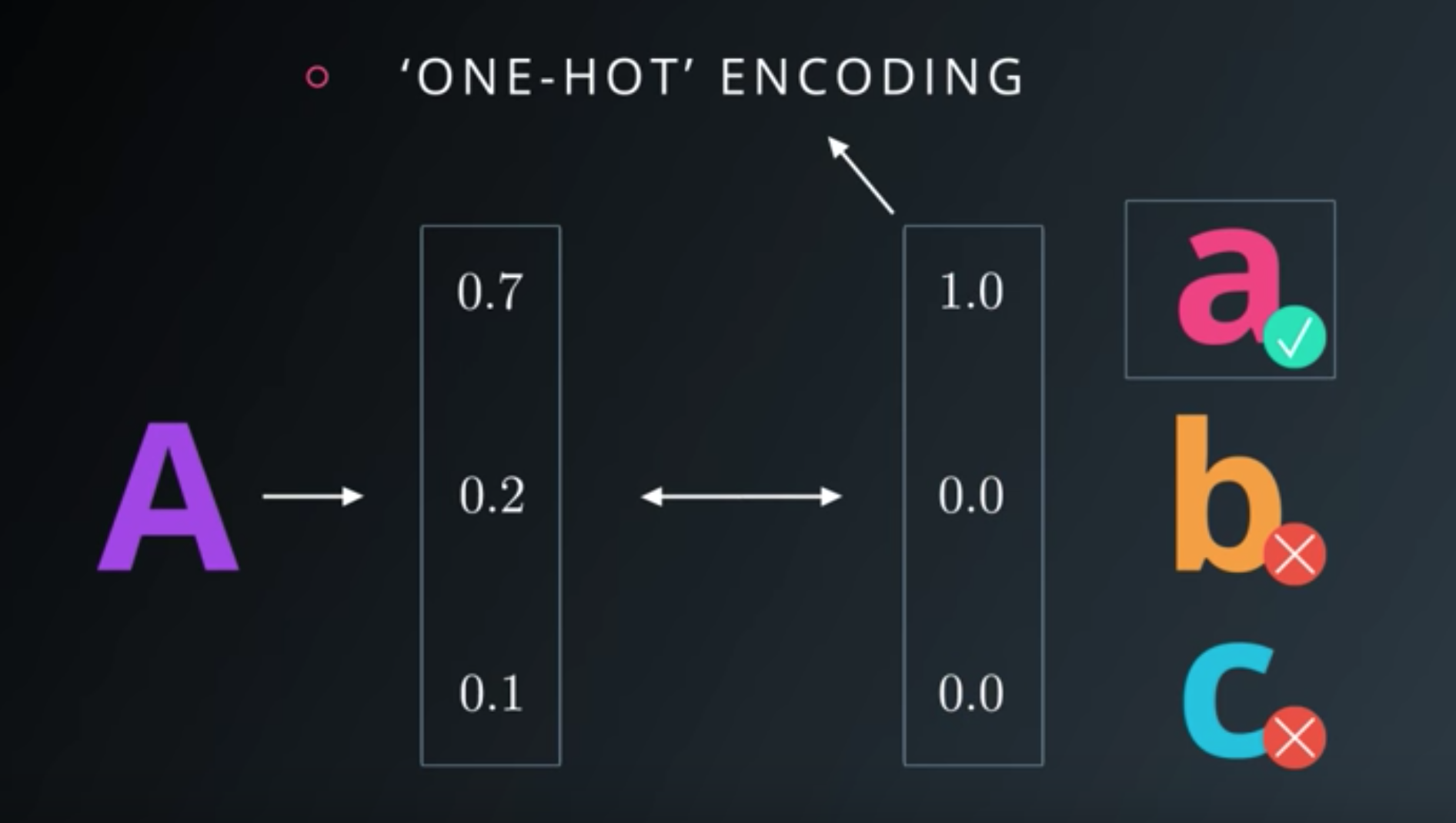
- You can also express your data labels as a vector using what’s called one-hot encoding.
- This just means that you have a vector the length of the number of classes, and the label element is marked with a
1while the other labels are set to0.
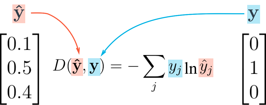
- We want our error to be proportional to how far apart these vectors are.
- To calculate this distance, we’ll use the cross entropy.
- Then, our goal when training the network is to make our prediction vectors as close as possible to the label vectors by minimizing the cross entropy.
Code:
import tensorflow as tf

softmax_data = [0.7, 0.2, 0.1]
one_hot_data = [1.0, 0.0, 0.0]

softmax = tf.placeholder(tf.float32)
one_hot = tf.placeholder(tf.float32)

# ToDo: Print cross entropy from session
cross_entropy = -tf.reduce_sum(tf.multiply(one_hot, tf.log(softmax)))

with tf.Session() as sess:
    print(sess.run(cross_entropy, feed_dict={softmax: softmax_data, one_hot: one_hot_data}))
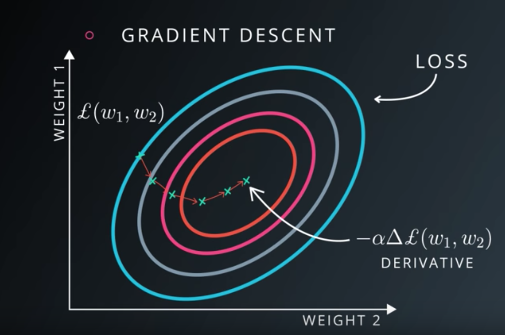
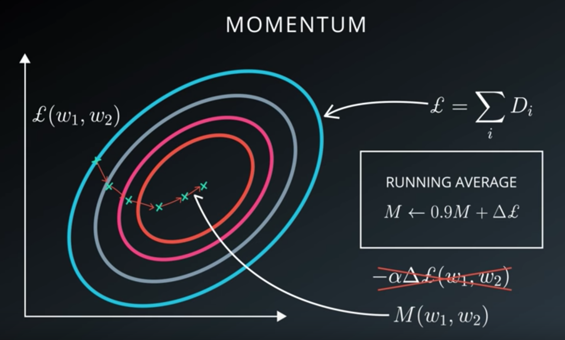
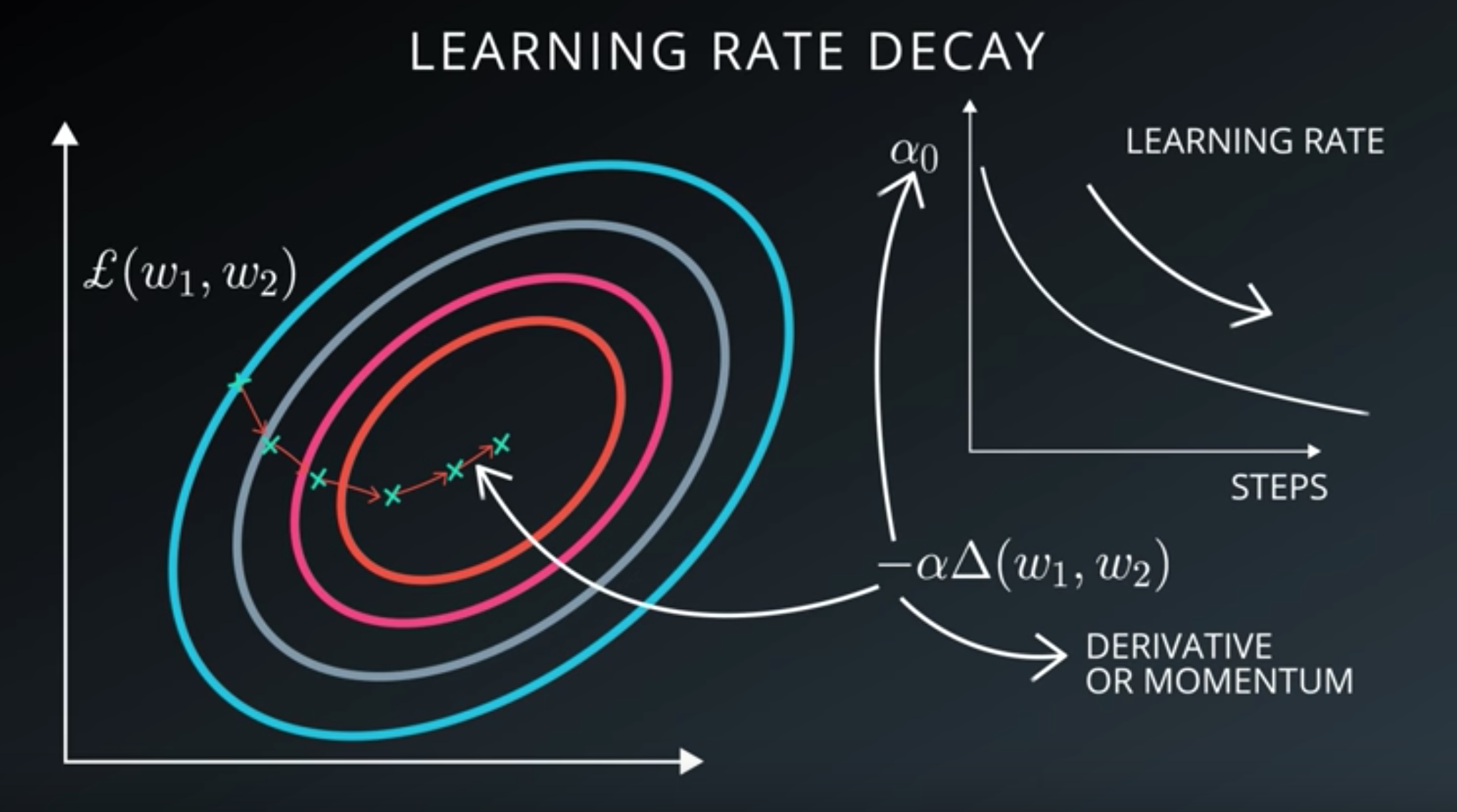
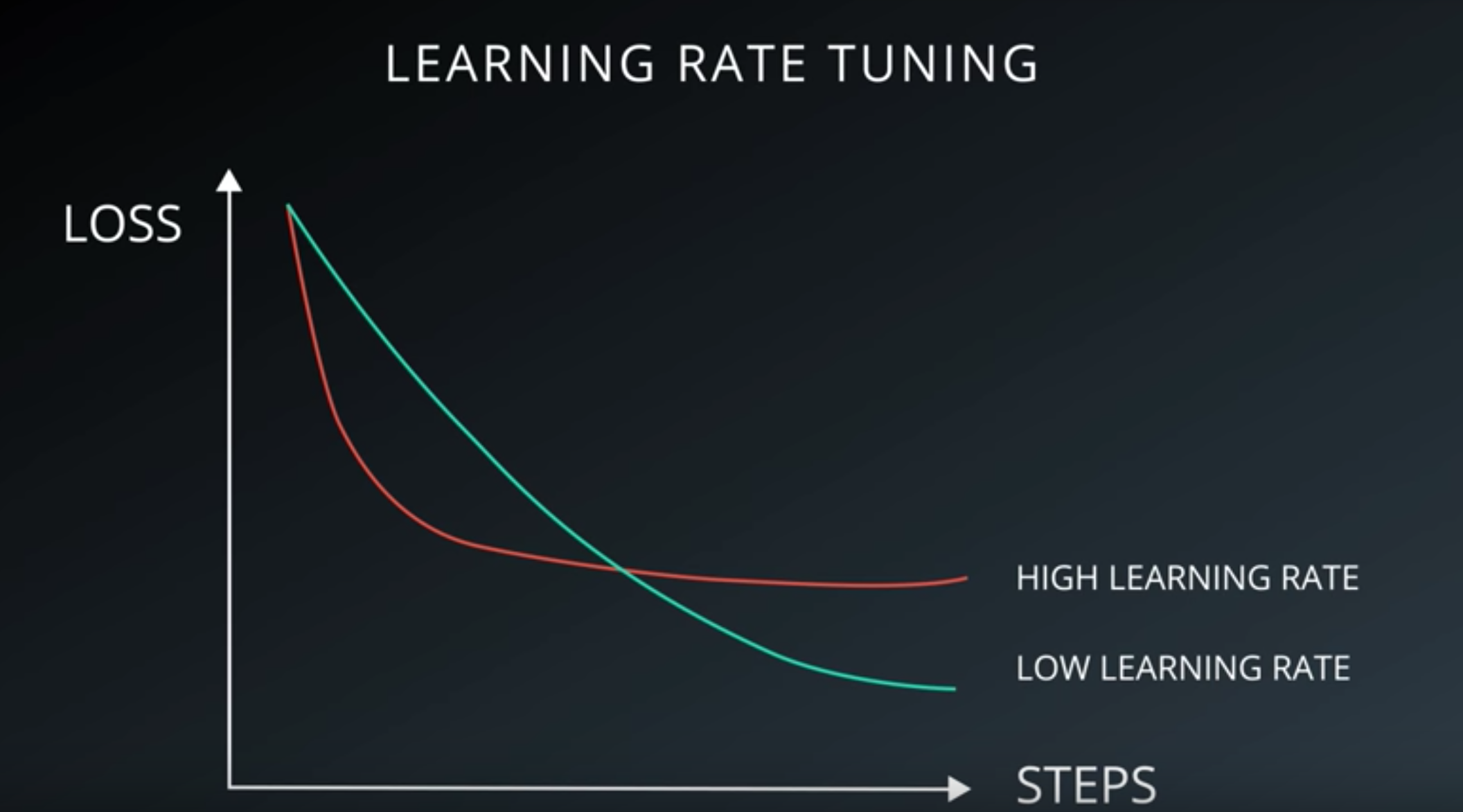
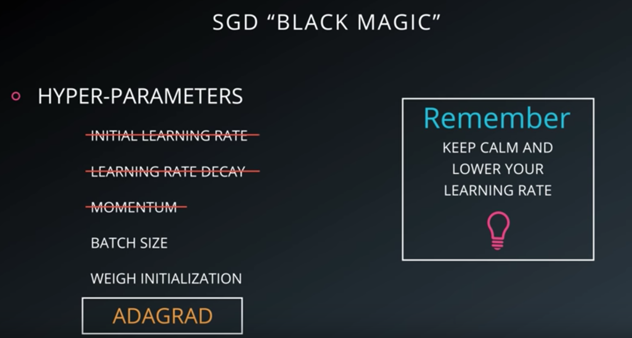
Minimizing Cross Entropy
Normalized Inputs and Initial Weights
Numerical Stability
- Adding very small values to a very large values can introduce a lot of errors.
a = 1000000000
for i in range(1000000):
    a = a + 0.000001
print(a - 1000000000)
>>>>>>>>>> 0.95367431640625

a = 1
for i in range(1000000):
    a = a + 0.000001
print(a - 1)
>>>>>>>>>> 0.9999999999177334
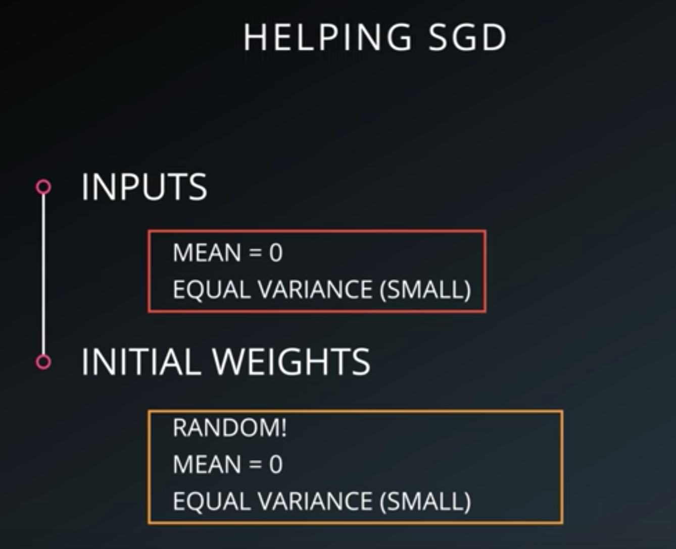
Normalized Inputs And Initial Weights
-
Initialization of weights, bias
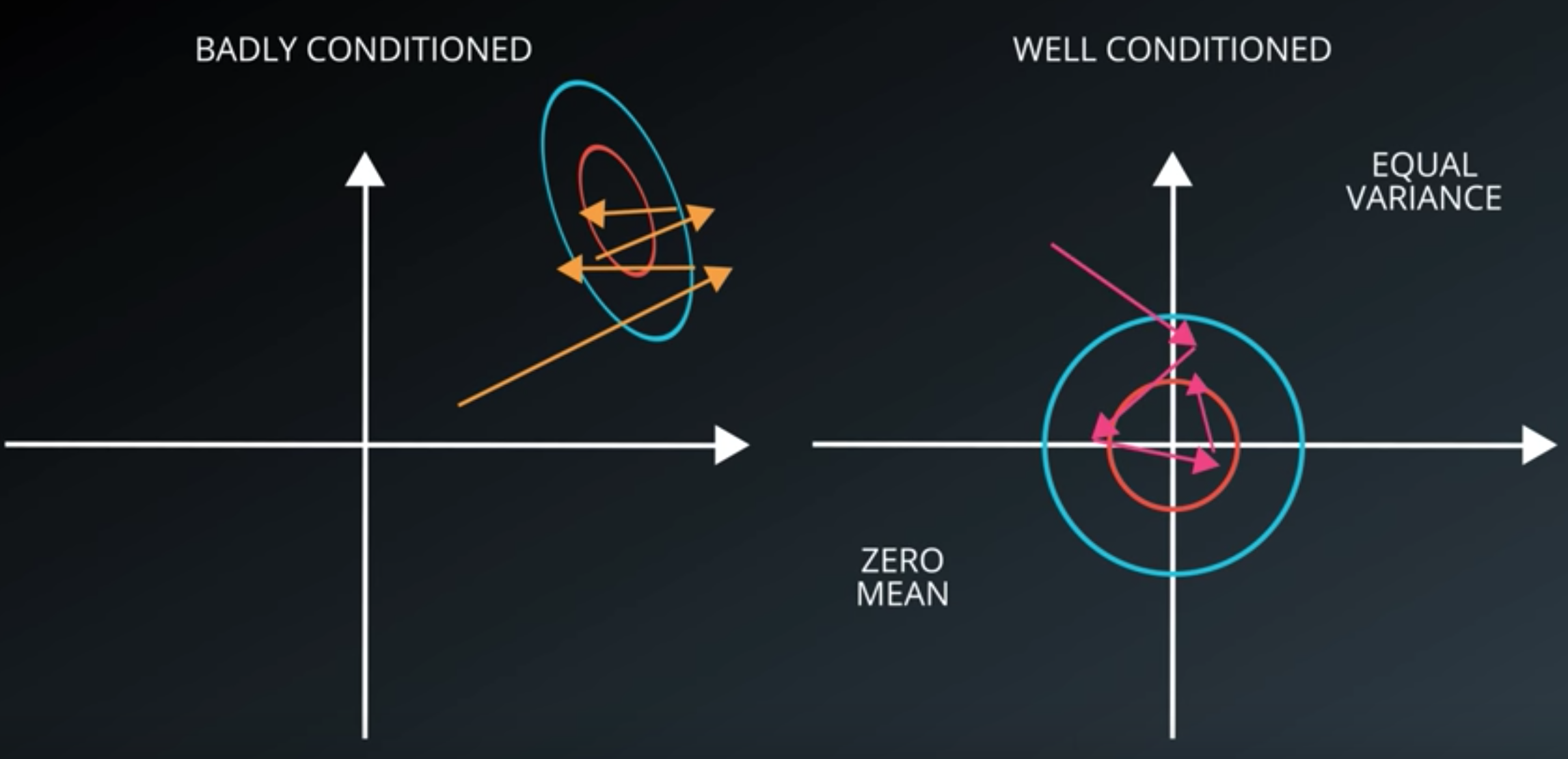
-
Initialization of the logic classifier
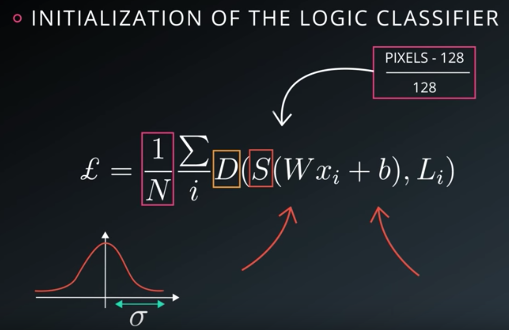
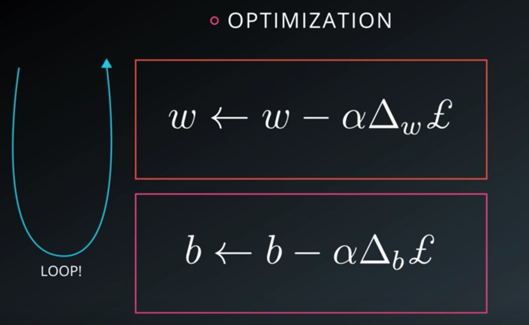
-
Optimization
Measuring Performance

Stochastic Gradient Descent
Mini-Batch
- Mini-batching is a technique for training on subsets of the dataset instead of all the data at one time.
- This provides the ability to train a model, even if a computer lacks the memory to store the entire dataset.
- Mini-batching is computationally inefficient, since you can’t calculate the loss simultaneously across all samples.
- However, this is a small price to pay in order to be able to run the model at all.
- It’s also quite useful combined with SGD.
- The idea is
- Randomly shuffle the data at the start of each epoch
- Then create the mini-batches.
- For each mini-batch, you train the network weights with gradient descent.
- Since these batches are random, you’re performing SGD with each batch.
Code batch:
def batches(batch_size, features, labels):
    """
    Create batches of features and labels
    :param batch_size: The batch size
    :param features: List of features
    :param labels: List of labels
    :return: Batches of (Features, Labels)
    """
    assert len(features) == len(labels)
    outout_batches = []

    sample_size = len(features)
    for start_i in range(0, sample_size, batch_size):
        end_i = start_i + batch_size
        batch = [features[start_i:end_i], labels[start_i:end_i]]
        outout_batches.append(batch)

    return outout_batches
Epochs
- An epoch is a single forward and backward pass of the whole dataset.
- This is used to increase the accuracy of the model without requiring more data.
Mini-Batch and Epochs in TensorFlow
from tensorflow.examples.tutorials.mnist import input_data
import tensorflow as tf
import numpy as np
from helper import batches  # Helper function created in Mini-batching section


def print_epoch_stats(epoch_i, sess, last_features, last_labels):
    """
    Print cost and validation accuracy of an epoch
    """
    current_cost = sess.run(
        cost,
        feed_dict={features: last_features, labels: last_labels})
    valid_accuracy = sess.run(
        accuracy,
        feed_dict={features: valid_features, labels: valid_labels})
    print('Epoch: {:<4} - Cost: {:<8.3} Valid Accuracy: {:<5.3}'.format(
        epoch_i,
        current_cost,
        valid_accuracy))

n_input = 784  # MNIST data input (img shape: 28*28)
n_classes = 10  # MNIST total classes (0-9 digits)

# Import MNIST data
mnist = input_data.read_data_sets('/datasets/ud730/mnist', one_hot=True)

# The features are already scaled and the data is shuffled
train_features = mnist.train.images
valid_features = mnist.validation.images
test_features = mnist.test.images

train_labels = mnist.train.labels.astype(np.float32)
valid_labels = mnist.validation.labels.astype(np.float32)
test_labels = mnist.test.labels.astype(np.float32)

# Features and Labels
features = tf.placeholder(tf.float32, [None, n_input])
labels = tf.placeholder(tf.float32, [None, n_classes])

# Weights & bias
weights = tf.Variable(tf.random_normal([n_input, n_classes]))
bias = tf.Variable(tf.random_normal([n_classes]))

# Logits - xW + b
logits = tf.add(tf.matmul(features, weights), bias)

# Define loss and optimizer
learning_rate = tf.placeholder(tf.float32)
cost = tf.reduce_mean(tf.nn.softmax_cross_entropy_with_logits(logits=logits, labels=labels))
optimizer = tf.train.GradientDescentOptimizer(learning_rate=learning_rate).minimize(cost)

# Calculate accuracy
correct_prediction = tf.equal(tf.argmax(logits, 1), tf.argmax(labels, 1))
accuracy = tf.reduce_mean(tf.cast(correct_prediction, tf.float32))

init = tf.global_variables_initializer()

batch_size = 128
epochs = 100
learn_rate = 0.001

train_batches = batches(batch_size, train_features, train_labels)

with tf.Session() as sess:
    sess.run(init)

    # Training cycle
    for epoch_i in range(epochs):

        # Loop over all batches
        for batch_features, batch_labels in train_batches:
            train_feed_dict = {
                features: batch_features,
                labels: batch_labels,
                learning_rate: learn_rate}
            sess.run(optimizer, feed_dict=train_feed_dict)

        # Print cost and validation accuracy of an epoch
        print_epoch_stats(epoch_i, sess, batch_features, batch_labels)

    # Calculate accuracy for test dataset
    test_accuracy = sess.run(
        accuracy,
        feed_dict={features: test_features, labels: test_labels})

print('Test Accuracy: {}'.format(test_accuracy))
Output:
Epoch: 90   - Cost: 0.105    Valid Accuracy: 0.869
Epoch: 91   - Cost: 0.104    Valid Accuracy: 0.869
Epoch: 92   - Cost: 0.103    Valid Accuracy: 0.869
Epoch: 93   - Cost: 0.103    Valid Accuracy: 0.869
Epoch: 94   - Cost: 0.102    Valid Accuracy: 0.869
Epoch: 95   - Cost: 0.102    Valid Accuracy: 0.869
Epoch: 96   - Cost: 0.101    Valid Accuracy: 0.869
Epoch: 97   - Cost: 0.101    Valid Accuracy: 0.869
Epoch: 98   - Cost: 0.1      Valid Accuracy: 0.869
Epoch: 99   - Cost: 0.1      Valid Accuracy: 0.869
Test Accuracy: 0.8696000006198883
- Lowering the learning rate would require more epochs, but could ultimately achieve better accuracy.