Convolutional Networks
Outline:
- Convolutional Networks
- Filters
- Strides and Padding
- Parameter Sharing
- Dimensionality
- TensorFlow Convolution Layer
- Advanced Convolution Network
- Pooling
- 1x1 Convolutions
- Inception Module
- Convolutional Network in TensorFlow
- Additional Resources
Convolutional Networks
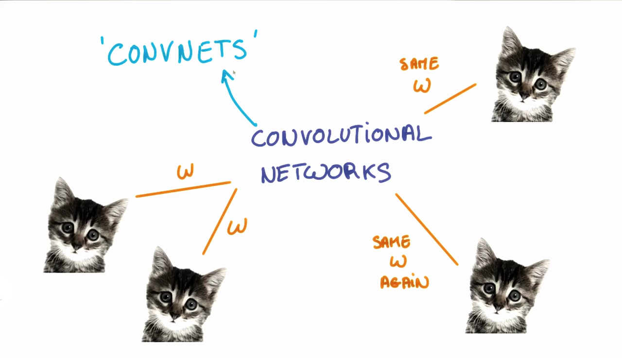
- Covnets(CNN) are neural networks that share their parameters across space.
CNNlearns to recognize basic lines and curves, then shapes and blobs, and then increasingly complex objects within the image.- Finally, the
CNNclassifies the image by combining the larger, more complex objects. - With deep learning, we don’t actually program the
CNNto recognize these specific features.- Rather, the
CNNlearns on its own to recognize such objects through forward propagation and backpropagation!
- Rather, the
- It’s amazing how well a
CNNcan learn to classify images, even though we never program theCNNwith information about specific features to look for.
Example:
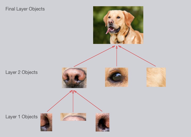
In our case, the levels in the hierarchy are:
- Simple shapes, like ovals and dark circles
- Complex objects (combinations of simple shapes), like eyes, nose, and fur
- The dog as a whole (a combination of complex objects)
Filters
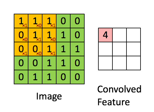
- The first step for a CNN is to break up the image into smaller pieces.
- We do this by selecting a width and height that defines a
filter.
- We do this by selecting a width and height that defines a
- The
filterlooks at small pieces, or patches, of the image. - Then simply slide this filter horizontally or vertically to focus on a different piece of the image.
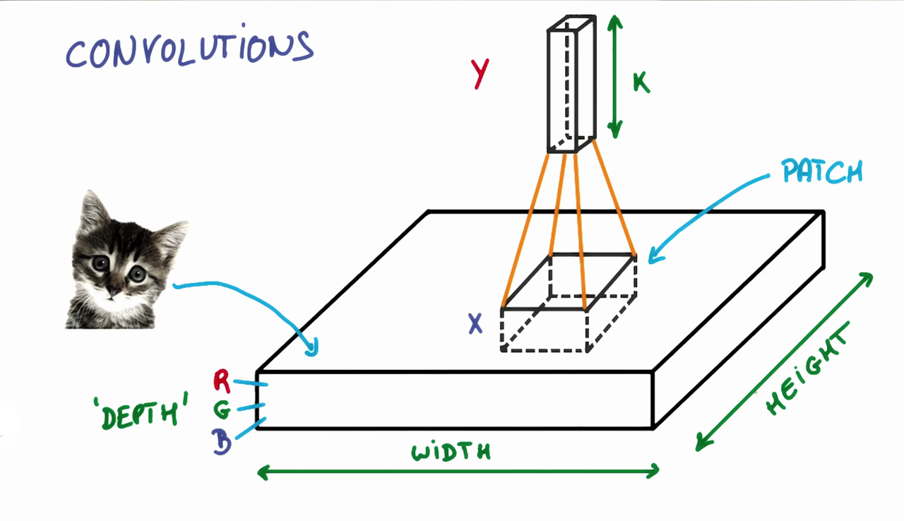
- It’s common to have more than one filter.
- Different filters pick up different qualities of a patch.
- For example, one filter might look for a particular color, while another might look for a kind of object of a specific shape.
- The amount of filters in a convolutional layer is called the
filter depth(k).- In practice, k is a hyperparameter we tune, and most CNNs tend to pick the same starting values.
- Multiple neurons can be useful because a patch can have multiple interesting characteristics that we want to capture.
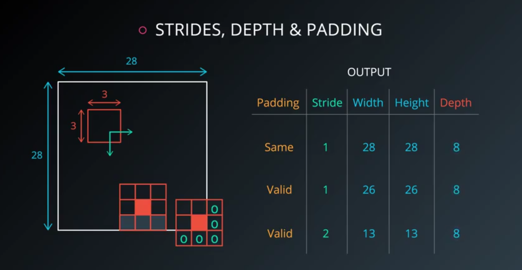
Strides and Padding
- The amount by which the filter slides is referred to as the
stride. - The
strideis a hyperparameter which you, the engineer, can tune.- Increasing the
stridereduces the size of your model by reducing the number of total patches each layer observes. - However, this usually comes with a reduction in accuracy.
- Increasing the
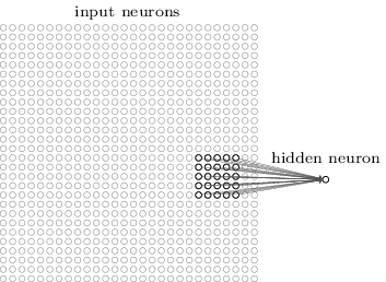
- In a normal, non-convolutional neural network, we would have ignored the adjacency.
Fully Connectedlayer is a standard, non convolutional layer, where all inputs are connected to all output neurons.- This is also referred to as a dense layer.
Parameter Sharing
- Trying to classify a picture of a cat, we don’t care where in the image a cat is.
- If it’s in the top left or the bottom right, it’s still a cat in our eyes.
- We would like our
CNNs to also possess this ability known as translation invariance.
- The weights and biases we learn for a given output layer are shared across all patches in a given input layer.
- Note that as we increase the depth of our filter, the number of weights and biases we have to learn still increases
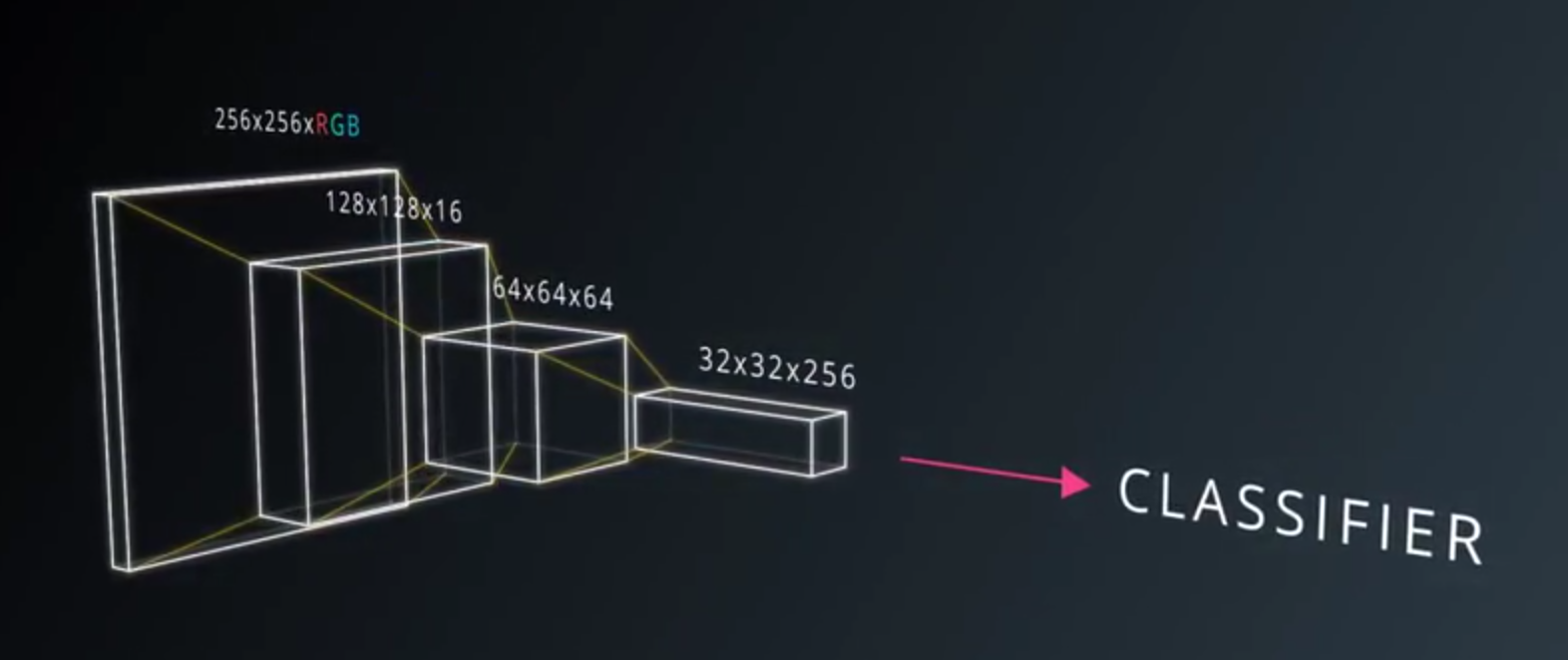
Dimensionality
From what we’ve learned so far, how can we calculate the number of neurons of each layer in our CNN?
Given:
- our input layer has a width of
Wand a height ofH - our convolutional layer has a filter size
F - we have a stride of
S - a padding of
P - and the number of filters
K,
Then:
- The following formula gives us the width of the next layer:
W_out =[ (W−F+2P)/S] + 1. - The output height would be
H_out = [(H-F+2P)/S] + 1. - And the output depth would be equal to the number of filters
D_out = K. - The output volume would be
W_out * H_out * D_out.
Knowing the dimensionality of each additional layer helps us understand how large our model is and how our decisions around filter size and stride affect the size of our network.
Dimensionality in Tensorflow
input = tf.placeholder(tf.float32, (None, 32, 32, 3))
filter_weights = tf.Variable(tf.truncated_normal((8, 8, 3, 20))) # (height, width, input_depth, output_depth)
filter_bias = tf.Variable(tf.zeros(20))
strides = [1, 2, 2, 1] # (batch, height, width, depth)
padding = 'SAME'
conv = tf.nn.conv2d(input, filter_weights, strides, padding) + filter_bias
- Note the output shape of conv will be
[1, 16, 16, 20].- It’s 4D to account for batch size, but more importantly, it’s not
[1, 14, 14, 20]. - This is because the padding algorithm TensorFlow uses is not exactly the same as the one above.
- An alternative algorithm is to switch padding from SAME to VALID which would result in an output shape of
[1, 13, 13, 20].
- It’s 4D to account for batch size, but more importantly, it’s not
In summary TensorFlow uses the following equation for SAME vs VALID
- SAME Padding, the output height and width are computed as:
out_height = ceil(float(in_height) / float(strides[1]))out_width = ceil(float(in_width) / float(strides[2]))
- VALID Padding, the output height and width are computed as:
out_height = ceil(float(in_height - filter_height + 1) / float(strides[1]))out_width = ceil(float(in_width - filter_width + 1) / float(strides[2]))
How many parameters?
- Setup
H = height, W = width, D = depth- We have an input of shape
32x32x3 (HxWxD) - 20 filters of shape
8x8x3 (HxWxD) - A stride of
2for both the height and width (S) - Zero padding of size
1 (P)
- Output Layer
14x14x20 (HxWxD)
- Quiz
- How many parameters does the convolutional layer have (without parameter sharing)?
(8 * 8 * 3 + 1) * (14 * 14 * 20) = 756560(we add 1 for the bias.)
- How many parameters does the convolution layer have (with parameter sharing)?
(8 * 8 * 3 + 1) * 20 = 3840 + 20 = 3860
- How many parameters does the convolutional layer have (without parameter sharing)?
TensorFlow Convolution Layer
TensorFlow provides the tf.nn.conv2d() and tf.nn.bias_add() functions to create your own convolutional layers.
# Output depth
k_output = 64

# Image Properties
image_width = 10
image_height = 10
color_channels = 3

# Convolution filter
filter_size_width = 5
filter_size_height = 5

# Input/Image
input = tf.placeholder(
    tf.float32,
    shape=[None, image_height, image_width, color_channels])

# Weight and bias
weight = tf.Variable(tf.truncated_normal(
    [filter_size_height, filter_size_width, color_channels, k_output]))
bias = tf.Variable(tf.zeros(k_output))

# Apply Convolution
conv_layer = tf.nn.conv2d(input, weight, strides=[1, 2, 2, 1], padding='SAME')
# Add bias
conv_layer = tf.nn.bias_add(conv_layer, bias)
# Apply activation function
conv_layer = tf.nn.relu(conv_layer)
strides = [batch, input_height, input_width, input_channels].- We are generally always going to set the stride for
batchandinput_channelsto be1.
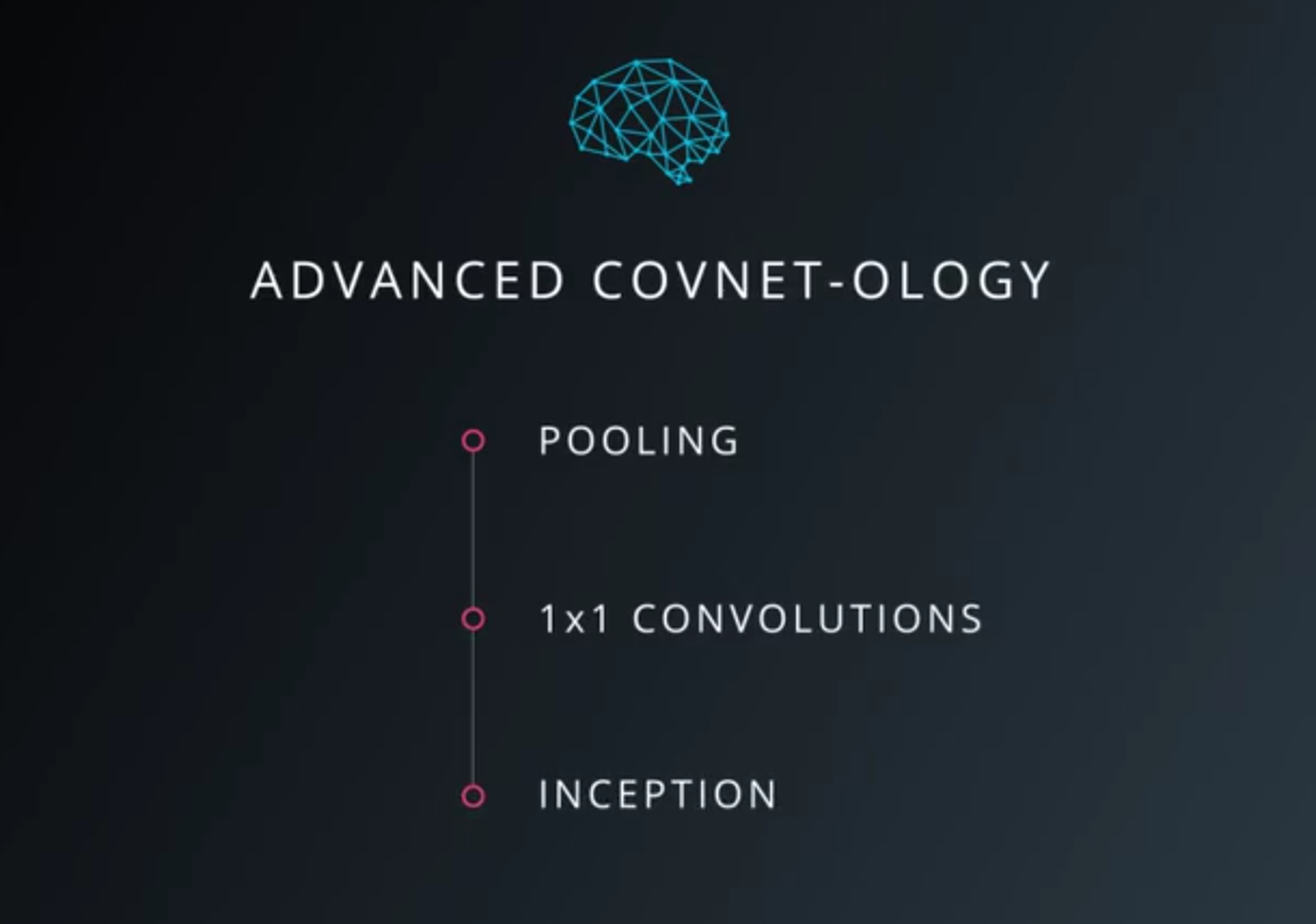
Advanced Convolution Network
There are many things we can improve CNN.
- Pooling
- 1x1 Convolutions
- Inception
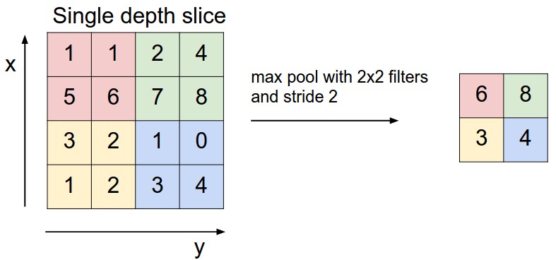
Pooling
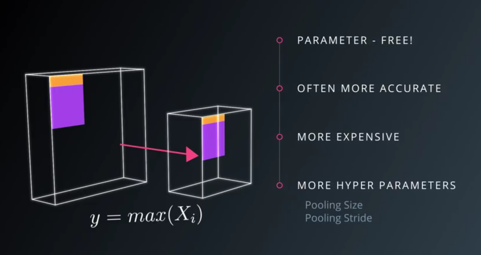
- Striding removes a lot of information.
- Pooling
- Convoltion strides
- Combine them somehow (max pooling, average pooling)
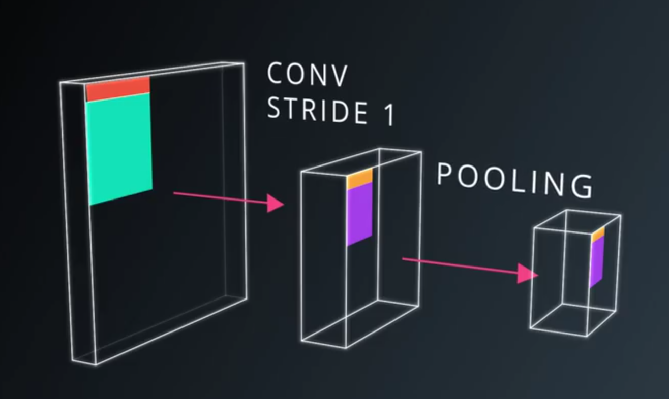
- A pooling layer is generally used to
- Decrease the size of the output
- Prevent overfitting
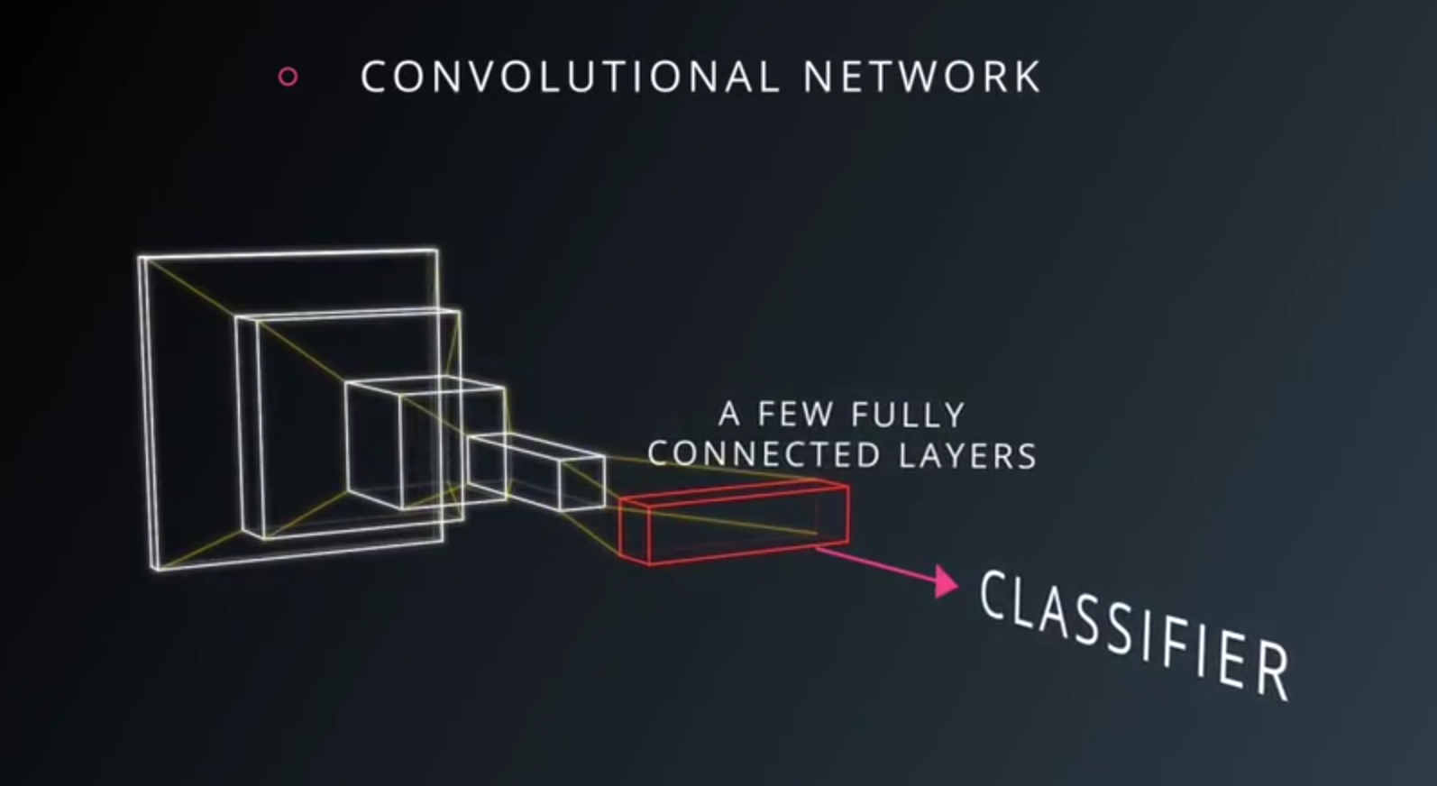
- Advantages of Max pooling
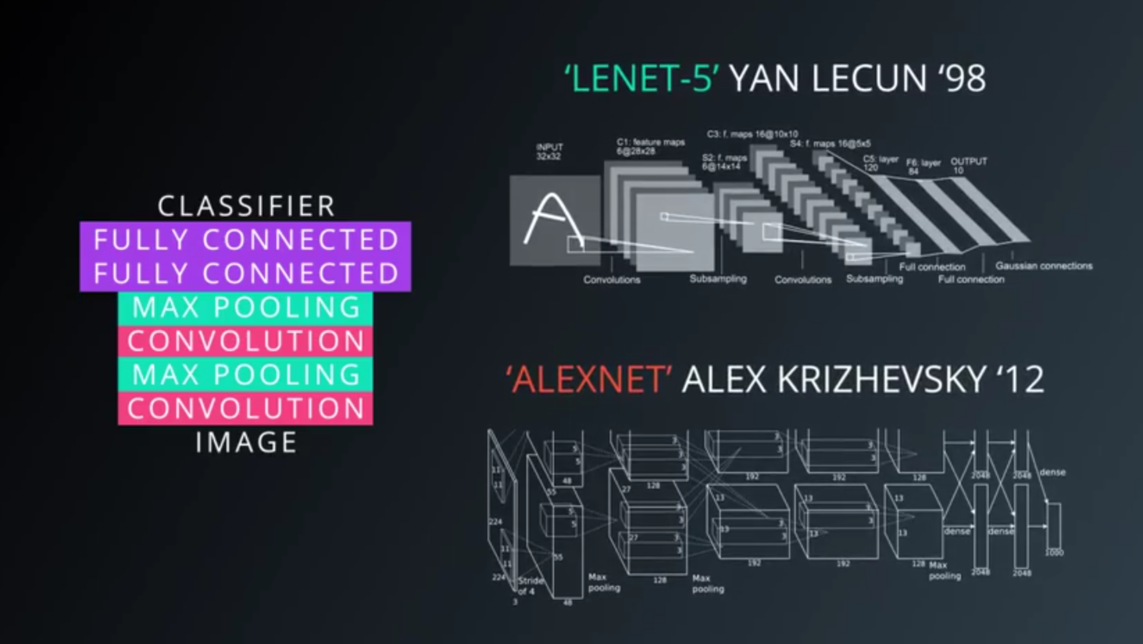
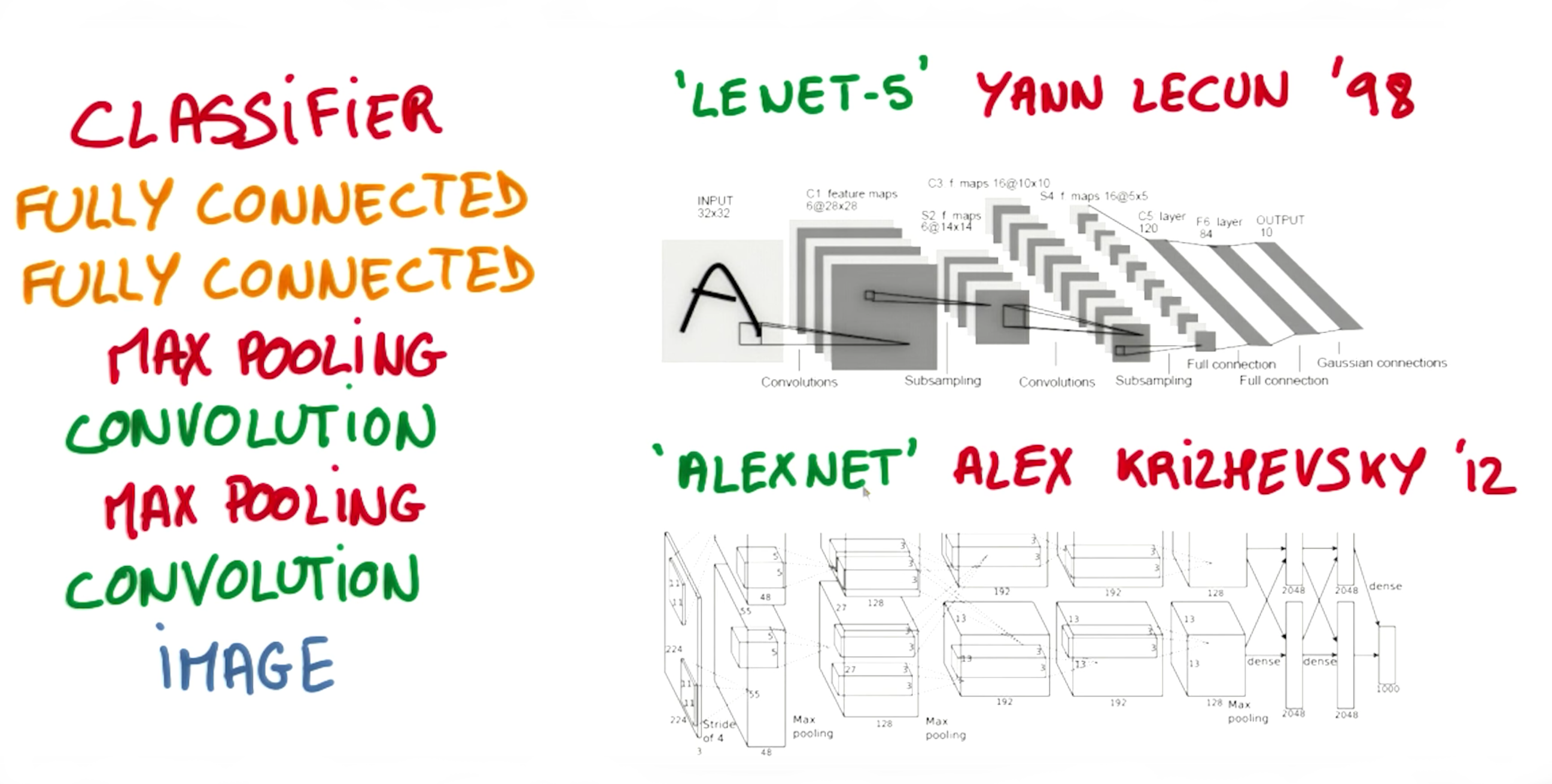
- A very typical architecture of a covnet
- a few layers alternating convolutions and max pooling
- a few fully connected layers at the top
- Famous models
- Recently, pooling layers have fallen out of favor. Some reasons are:
- Recent datasets are so big and complex we’re more concerned about underfitting.
- Dropout is a much better regularizer.
- Pooling results in a loss of information. Think about the max pooling operation as an example. We only keep the largest of n numbers, thereby disregarding n-1 numbers completely.
TensorFlow Max Pooling
...
conv_layer = tf.nn.conv2d(input, weight, strides=[1, 2, 2, 1], padding='SAME')
conv_layer = tf.nn.bias_add(conv_layer, bias)
conv_layer = tf.nn.relu(conv_layer)
# Apply Max Pooling
conv_layer = tf.nn.max_pool(
    conv_layer,
    ksize=[1, 2, 2, 1],
    strides=[1, 2, 2, 1],
    padding='SAME')
- The
tf.nn.max_pool()function performs max pooling- with the
ksizeparameter as the size of the filter - and the
stridesparameter as the length of the stride. 2x2filters with a stride of2x2are common in practice.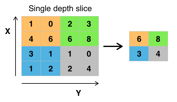
- with the
- The ksize and strides parameters are structured as 4-element lists
[batch, height, width, channels]- the batch and channel dimensions are typically set to
1.
1x1 Convolutions
1x1 Convolutionsis basically a small classifier for patch of the image.- It is only linear classifier.
- If we add
1x1 Convolutionsin the middle- Suddenly we have mini neural network running over the patch.
- Instead of linear classifier.
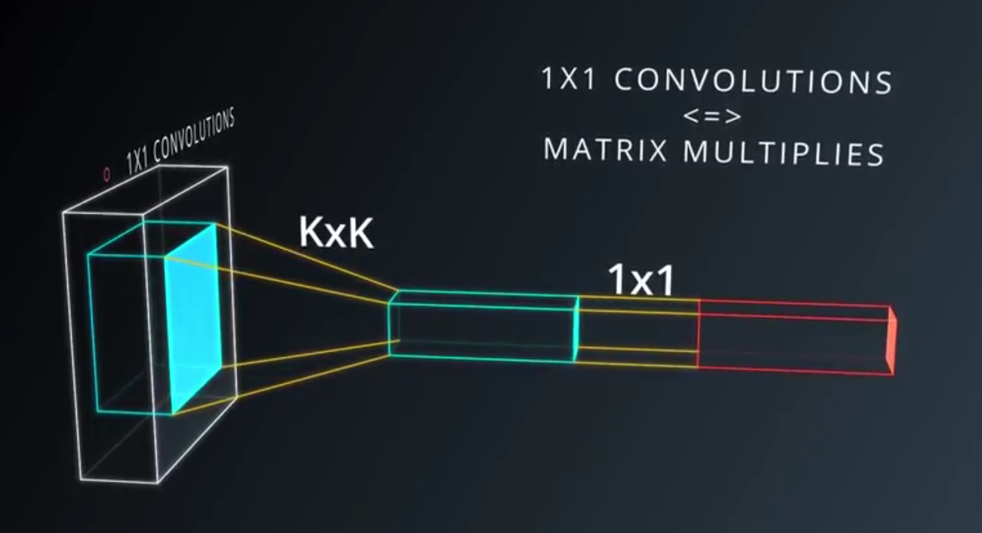
- Interspersing
1x1 Convolutions- Very inexpensive way to make models to deeper and have more parameters
- Without completely changing their structure.
- It is just matrix multiply.
Inception Module
- Inception Module, each layer of the covnet, we can make a choice!
- Pooling? or 1x1 Convolution?
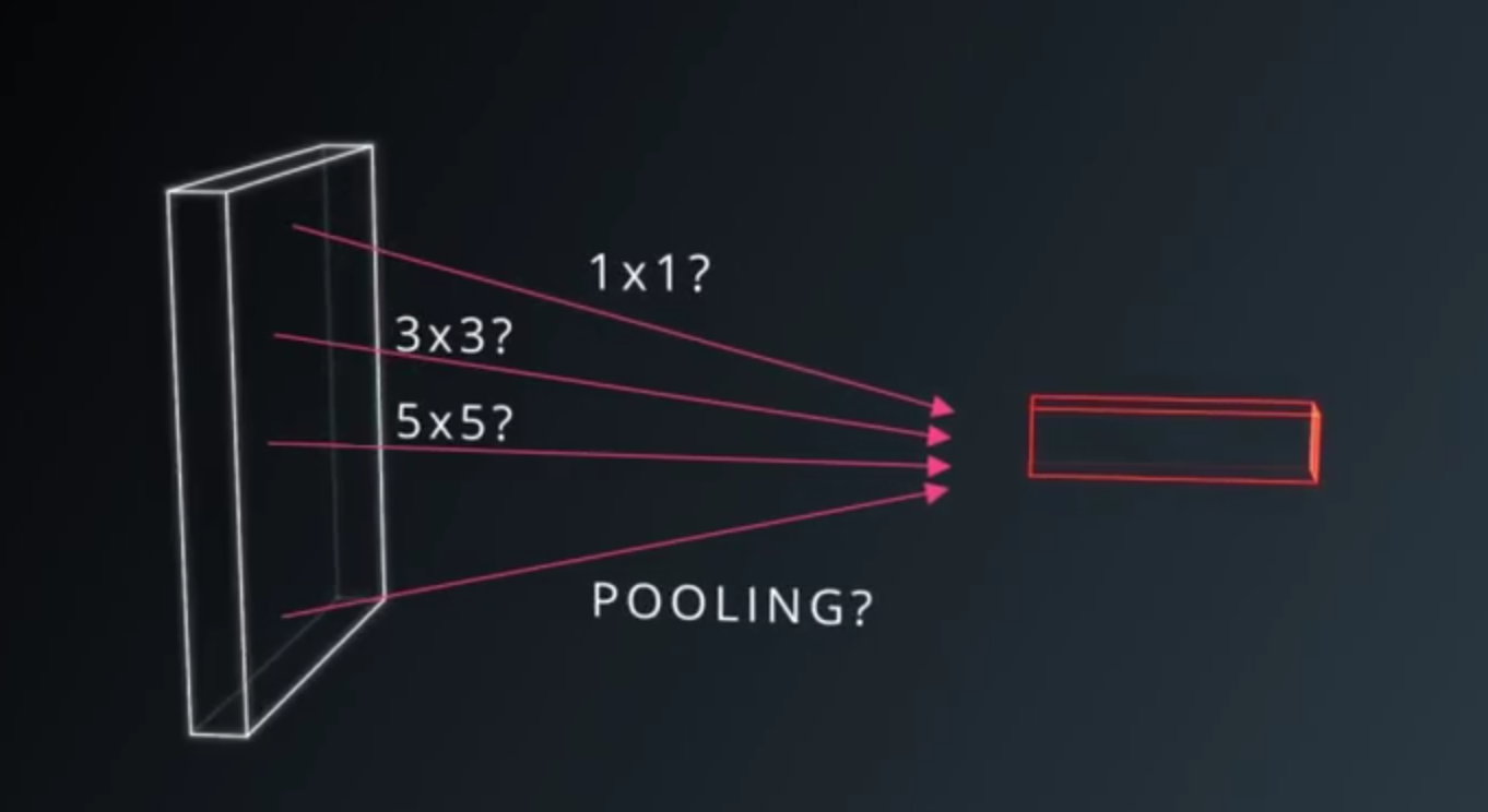
- All these choices are beneficial to the modeling power
- Why choose? Use them All
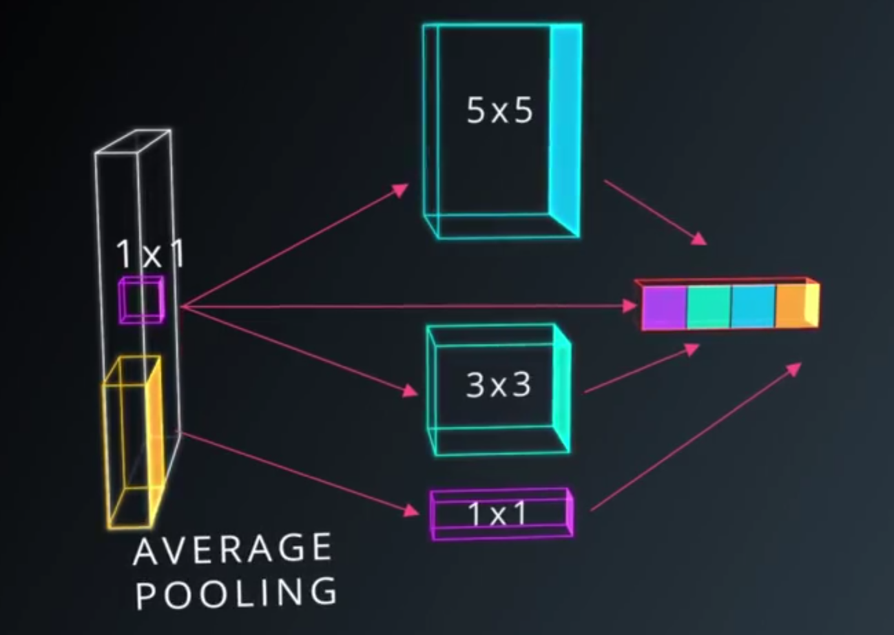
- Pooling? or 1x1 Convolution?
- We can choose these parameters, total parameters in our model is very small
- Model performs better than simple convolution.
Convolutional Network in TensorFlow
The structure of this network follows the classic structure of CNNs, which is a mix of
- convolutional layers
- and max pooling,
- followed by fully-connected layers.
Dataset
from tensorflow.examples.tutorials.mnist import input_data
mnist = input_data.read_data_sets(".", one_hot=True, reshape=False)

import tensorflow as tf

# Parameters
learning_rate = 0.00001
epochs = 10
batch_size = 128

# Number of samples to calculate validation and accuracy
# Decrease this if you're running out of memory to calculate accuracy
test_valid_size = 256

# Network Parameters
n_classes = 10  # MNIST total classes (0-9 digits)
dropout = 0.75  # Dropout, probability to keep units
Weights and Biases
# Store layers weight & bias
weights = {
    'wc1': tf.Variable(tf.random_normal([5, 5, 1, 32])),
    'wc2': tf.Variable(tf.random_normal([5, 5, 32, 64])),
    'wd1': tf.Variable(tf.random_normal([7*7*64, 1024])),
    'out': tf.Variable(tf.random_normal([1024, n_classes]))}

biases = {
    'bc1': tf.Variable(tf.random_normal([32])),
    'bc2': tf.Variable(tf.random_normal([64])),
    'bd1': tf.Variable(tf.random_normal([1024])),
    'out': tf.Variable(tf.random_normal([n_classes]))}
Convolutions
def conv2d(x, W, b, strides=1):
    x = tf.nn.conv2d(x, W, strides=[1, strides, strides, 1], padding='SAME')
    x = tf.nn.bias_add(x, b)
    return tf.nn.relu(x)
Max Pooling
def maxpool2d(x, k=2):
    return tf.nn.max_pool(
        x,
        ksize=[1, k, k, 1],
        strides=[1, k, k, 1],
        padding='SAME')
Model
def conv_net(x, weights, biases, dropout):
    # Layer 1 - 28*28*1 to 14*14*32
    conv1 = conv2d(x, weights['wc1'], biases['bc1'])
    conv1 = maxpool2d(conv1, k=2)

    # Layer 2 - 14*14*32 to 7*7*64
    conv2 = conv2d(conv1, weights['wc2'], biases['bc2'])
    conv2 = maxpool2d(conv2, k=2)

    # Fully connected layer - 7*7*64 to 1024
    fc1 = tf.reshape(conv2, [-1, weights['wd1'].get_shape().as_list()[0]])
    fc1 = tf.add(tf.matmul(fc1, weights['wd1']), biases['bd1'])
    fc1 = tf.nn.relu(fc1)
    fc1 = tf.nn.dropout(fc1, dropout)

    # Output Layer - class prediction - 1024 to 10
    out = tf.add(tf.matmul(fc1, weights['out']), biases['out'])
    return out
Session
# tf Graph input
x = tf.placeholder(tf.float32, [None, 28, 28, 1])
y = tf.placeholder(tf.float32, [None, n_classes])
keep_prob = tf.placeholder(tf.float32)

# Model
logits = conv_net(x, weights, biases, keep_prob)

# Define loss and optimizer
cost = tf.reduce_mean(\
    tf.nn.softmax_cross_entropy_with_logits(logits=logits, labels=y))
optimizer = tf.train.GradientDescentOptimizer(learning_rate=learning_rate)\
    .minimize(cost)

# Accuracy
correct_pred = tf.equal(tf.argmax(logits, 1), tf.argmax(y, 1))
accuracy = tf.reduce_mean(tf.cast(correct_pred, tf.float32))

# Initializing the variables
init = tf. global_variables_initializer()

# Launch the graph
with tf.Session() as sess:
    sess.run(init)

    for epoch in range(epochs):
        for batch in range(mnist.train.num_examples//batch_size):
            batch_x, batch_y = mnist.train.next_batch(batch_size)
            sess.run(optimizer, feed_dict={
                x: batch_x,
                y: batch_y,
                keep_prob: dropout})

            # Calculate batch loss and accuracy
            loss = sess.run(cost, feed_dict={
                x: batch_x,
                y: batch_y,
                keep_prob: 1.})
            valid_acc = sess.run(accuracy, feed_dict={
                x: mnist.validation.images[:test_valid_size],
                y: mnist.validation.labels[:test_valid_size],
                keep_prob: 1.})

            print('Epoch {:>2}, Batch {:>3} -'
                  'Loss: {:>10.4f} Validation Accuracy: {:.6f}'.format(
                epoch + 1,
                batch + 1,
                loss,
                valid_acc))

    # Calculate Test Accuracy
    test_acc = sess.run(accuracy, feed_dict={
        x: mnist.test.images[:test_valid_size],
        y: mnist.test.labels[:test_valid_size],
        keep_prob: 1.})
    print('Testing Accuracy: {}'.format(test_acc))
Additional Resources
These are the resources we recommend in particular:
- Andrej Karpathy’s CS231n Stanford course on Convolutional Neural Networks.
- Michael Nielsen’s free book on Deep Learning.
- Goodfellow, Bengio, and Courville’s more advanced free book on Deep Learning.